Optimal Policy Rules in HANK

†

Alisdair McKay Christian K. Wolf

FRB Minneapolis MIT & NBER

March 13, 2023

Abstract: We characterize optimal policy rules in business-cycle models with

nominal rigidities and heterogeneous households. The derived rules are expressed

in terms of the causal eﬀects of policy instruments on policymaker targets. Our

ﬁrst result is that the optimal policy rule of a “dual mandate” central banker—a

policymaker that only cares about inﬂation and output—is unaﬀected by house-

hold heterogeneity. The optimal rule of a Ramsey planner contains an additional

distributional term that incorporates the eﬀects of her available policy instru-

ments on consumption inequality. We quantify the role of this term in a structural

model that incorporates and is consistent with evidence on the key distributional

channels of monetary policy, and we ﬁnd that the concern for inequality only

has a moderate eﬀect on optimal interest rate policy. Fiscal stimulus payments,

on the other hand, have strongly progressive eﬀects and are thus well-suited to

cushion the distributional eﬀects of cyclical ﬂuctuations.

†

Email: [email protected] and [email protected]. We thank Adrien Auclert, Anmol Bhan-

dari, Jordi Gal´ı,

Emilien Gouin-Bonenfant, and Ludwig Straub for helpful comments. The views expressed

herein are those of the authors and not necessarily those of the Federal Reserve Bank of Minneapolis or the

Federal Reserve System.

1 Introduction

Should household inequality aﬀect the conduct of cyclical stabilization policy? Recent years

have seen a surge of interest in this question, with several prominent studies arguing that the

design of optimal monetary policy is substantially altered by distributional considerations

(e.g., Bhandari et al., 2021; Acharya et al., 2022). In principle, household heterogeneity can

aﬀect optimal policy design in two separate ways. First, household inequality could alter the

transmission from policy instruments to any given target (e.g., inﬂation and output). This

change in transmission may aﬀect whether or not a policymaker can attain her given targets,

and how policy instruments need to be set to do so. Second, household heterogeneity may

also alter the targets themselves. For example, with market incompleteness, policymakers

may want to dampen the distributional eﬀects of cyclical ﬂuctuations.

We provide new insights into this question by expressing optimal policy rules in business-

cycle models with household heterogeneity in terms of empirically measurable “suﬃcient

statistics.” Our ﬁrst contribution is to cast optimal policy problems in a rich heterogeneous-

agent New Keynesian (HANK) environment in linear-quadratic form, closely mirroring the

canonical representative-agent New Keynesian (RANK) literature. As familiar from this lit-

erature, the solution to the linear-quadratic policy problem takes the form of a forecast target

criterion, providing a general characterization of optimal policy completely independently of

the shocks hitting the economy (Giannoni & Woodford, 2002). Drawing on McKay & Wolf

(2023), we furthermore show that these optimal policy rules can be expressed in terms of the

dynamic causal eﬀects of policy instruments on policymaker targets. This “suﬃcient statis-

tics” characterization of optimal policy rules has two beneﬁts. First, it provides a convenient

organizing device for understanding the literature—diﬀerences in optimal policy design can

be traced back to diﬀerences in the causal eﬀects of the policy instrument on policymaker

targets. Second, it suggests a natural avenue for model discipline—connect as tightly as

possible with existing empirical evidence on the causal eﬀects of policy interventions.

We then use our suﬃcient statistics framework to revisit the two ways in which household

heterogeneity can in principle aﬀect optimal policy design. On transmission (i.e., ﬁxing

policymaker targets), we show that the optimal policy rule of a dual mandate central banker

does not change with household heterogeneity. Such heterogeneity may aﬀect the path of

interest rates required to implement the dual mandate optimum, but our suﬃcient statistics

perspective reveals that the scope even for this is rather limited. On targets, in principle,

distributional concerns can have large eﬀects on optimal stabilization policy. In practice,

however, empirical evidence suggests that monetary policy has broad-based eﬀects in the

cross-section of households, with consumption of all households rising following a monetary

easing, and vice-versa. Monetary policy is thus a rather blunt distributional tool, and as a

result a Ramsey planner in an environment consistent with such broad-based eﬀects does

not choose to deviate much from dual mandate policy prescriptions.

Environment. Our analysis is set in a business-cycle model with nominal rigidities and

household heterogeneity. Households face idiosyncratic income risk and self-insure by bor-

rowing and saving in capital, short-term bonds, and long-term bonds. The policymaker sets

short-term nominal interest rates, pays transfers to households, and ﬁnances its expenditure

through taxation as well as bond issuance. As we discuss later, the environment is designed

to be rich enough to speak to the core channels of how monetary policy aﬀects consumption

across the cross-section of households.

In this environment we study optimal policy problems cast in linear-quadratic form (e.g.,

Giannoni & Woodford, 2002; Benigno & Woodford, 2012). Linearization of the private-

sector relations of our economy yields the linear constraints. Our quadratic objective is then

either ad hoc—a conventional dual mandate objective—or derived as an approximation to a

particular Ramsey policy problem.

Dual-mandate central banker. We begin our analysis by studying the optimal policy

problem of a conventional “dual-mandate” central banker that seeks to close the output gap

and stabilize inﬂation. We ﬁnd this ad hoc loss function useful as a starting point, for two

reasons. First, conceptually, it allows us to explore the eﬀects of changes in policy instrument

propagation while ﬁxing policymaker targets. Second, practically, it is arguably the relevant

objective function for real-world central banks.

Our main result is that the optimal interest rate target criterion for such a dual mandate

central banker is exactly the same as in a standard representative-agent environment. The

logic is as follows. Household heterogeneity in our environment only aﬀects the demand side

of the economy (i.e., the model’s “IS” curve). In the optimal policy problem, however, this

demand block is a slack constraint: the policymaker can pick an output-inﬂation allocation

subject to the Phillips curve, and then set nominal interest rates as necessary to generate

demand consistent with the desired allocation. Household heterogeneity thus may matter

for the path of the policy instrument, but not for optimal output and inﬂation outcomes.

Leveraging our suﬃcient statistics perspective, we then connect these theoretical results

on optimal dual-mandate policy to empirical evidence on monetary policy shock transmis-

sion. The empirical literature has tried to identify the causal eﬀects of nominal rate changes

on output and inﬂation (e.g. see Ramey, 2016). While silent on transmission mechanisms

and so in particular on the importance of heterogeneity-related channels, aggregate data are

informative about the size of interest rate movements required to move output and inﬂa-

tion by a given amount. But it then follows that quantitatively relevant HANK and RANK

models—that is, models that are consistent with the empirical evidence on monetary shock

propagation—will not only share the same optimal dual-mandate policy rule, but they will

in fact also tend to agree quite closely on the interest rate path needed to implement the

optimal inﬂation and output outcomes. Our quantitative analysis conﬁrms this insight: our

HANK model—which is calibrated to agree with this empirical evidence on monetary shock

propagation—agrees closely with a RANK model calibrated to the same evidence.

Ramsey problem. We next study a Ramsey problem in which the planner seeks to max-

imize a weighted sum of individual household utilities, allowing us to explore the role of

changes in policymaker objectives. Applying a second order approximation, we derive a loss

function that adds to the usual output gap and inﬂation objectives a third term reﬂect-

ing distributional concerns. We then solve the policymaker problem of minimizing this loss

function subject to linearized private-sector optimality conditions.

The policymaker’s problem now yields an optimal policy rule consisting of three terms,

trading oﬀ the policymaker’s ability to use her policy instrument to stabilize output, inﬂa-

tion, and the cross-sectional consumption distribution. The third term of this rule—which,

importantly, is the sole diﬀerence from the optimal standard dual mandate policy rule—is

governed by the distributional incidence of the instrument. If, for example, interest rate

movements do not aﬀect consumption shares (e.g., as in Werning, 2015), then the third term

is zero and the Ramsey rule is identical to the optimal dual-mandate rule; if, on the other

hand, monetary policy has large distributional eﬀects (e.g., as in Bhandari et al., 2021), then

distributional concerns may swamp price and output stability considerations.

To characterize the quantitatively relevant Ramsey policy, we again leverage our suﬃcient

statistics perspective. As we have discussed, our conclusions on optimal policy will be

governed by the causal eﬀects of interest rate policy on consumption inequality. Since prior

empirical work has delivered the sharpest results on the cross-sectional income incidence of

monetary policy, our strategy is to calibrate our model to match these distributional channels

of monetary policy, and then rely on the structure of the model to infer the ultimate eﬀects on

consumption inequality. Two features of our model turn out to be particularly relevant. First,

our model features long-duration assets, allowing us to capture an important redistribution

channel of monetary policy (see Auclert, 2019). Second, the model is designed to generate

only a modest response of aggregate labor income following a monetary expansion, consistent

with empirical evidence. For our purposes, the key takeaway is that the model generates

fairly evenly distributed eﬀects of policy, with consumption responding by similar percentage

amounts across the wealth and income distribution. Given this particular incidence, we ﬁnd

that monetary policy is rather ill-suited as a tool to deal with the distributional implications

of business-cycle shocks. For example, if—in response to a shock that largely aﬀects the

consumption of the poor—interest rates were set to stabilize consumption at the bottom,

then consumption of other households and so aggregate output and inﬂation would overshoot.

The Ramsey policymaker does not ﬁnd such overshooting optimal, and instead responds to

the shock similarly to conventional optimal dual-mandate policy. These quantitative ﬁndings

contrast with recent work on optimal monetary policy with heterogeneous households that

tends to ﬁnd an important role for distributional considerations (e.g., Bhandari et al., 2021;

Acharya et al., 2022; D´avila & Schaab, 2022).

Finally, we also brieﬂy consider a Ramsey policymaker that jointly sets interest rates and

stimulus checks, consistent with recent U.S. policy practice. While equivalent in their eﬀects

on output and inﬂation (Wolf, 2021), the two instruments diﬀer signiﬁcantly in their distribu-

tional incidence, with ﬁscal stimulus payments sharply compressing consumption inequality.

The two instruments are thus highly complementary, with monetary policy primarily aimed

at aggregate stabilization while ﬁscal policy manages distributional concerns.

Literature. We contribute to the literature on optimal policy in business-cycle models

with rich microeconomic heterogeneity (Acharya et al., 2022; Bhandari et al., 2021; Le Grand

et al., 2022; D´avila & Schaab, 2022). Conceptually, our key contribution is to characterize

optimal policy through forecast target criteria expressed in terms of easily interpretable suf-

ﬁcient statistics. Our computation of these optimal policy rules leverages sequence-space

representations of equilibria and thus the recent work of Auclert et al. (2021).

A con-

temporaneous paper that does the same is D´avila & Schaab (2022). Those authors do not

rely on linear-quadratic approximations, thus providing more general optimal policy results,

but without our suﬃcient statistics perspective. Our discussion of the mapping between

By the equivalence of perfect-foresight sequence-space and stochastic linear state-space methods, our tar-

geting criterion also applies to the analogous stochastic linear-quadratic optimal control problem. Sequence-

space linear-quadratic policy problems have been used in prior work to derive “optimal policy projections”

(Svensson, 2005; De Groot et al., 2021; Hebden & Winker, 2021).

policy rules and empirical evidence builds on our earlier work in McKay & Wolf (2023).

These conceptual innovations allow us to revisit several substantive results in the prior

heterogeneous-household optimal policy literature.

First, we derive a sharp set of irrelevance results for the eﬀects of inequality on optimal

policy design. Prior work has emphasized that inequality will aﬀect policy propagation by

altering the demand side of the economy (Kaplan et al., 2018; Auclert, 2019); our analysis,

however, reveals that these changes do not aﬀect the optimal “dual mandate” output and in-

ﬂation outcomes. If furthermore matched to the same evidence on policy shock propagation,

then HANK and RANK models will also (roughly) agree on the required rate paths.

Second, our suﬃcient statistics perspective provides novel insights on the insurance role

of stabilization policy. Our formulation of the Ramsey problem objective isolates the pol-

icymaker’s desire to provide insurance against aggregate shocks with unequal incidence on

consumption across households.

In particular, our second-order approximation to the social

welfare function extends a similar ﬁnding by Acharya et al. to a more traditional HANK

model that does not permit analytical aggregation. The key beneﬁt of our formulation is that

it delivers a transparent characterization of optimal policy, with the extent to which house-

hold heterogeneity aﬀects the optimal Ramsey policy fully governed by the distributional

eﬀects of the policy instrument. Guided by these insights, and diﬀerently from prior work

(e.g., Bhandari et al., 2021; Le Grand et al., 2022), we consider a rich quantitative model

that is consistent with the main distributional channels of monetary stabilization policy.

Finally, our analysis of optimal joint ﬁscal-monetary policy extends results in Wolf (2021)

and Bilbiie et al. (2021). Wolf (2021) shows that, in a standard HANK setting, transfers and

monetary policy can implement the same aggregate allocations, but diﬀer in their distribu-

tional implications. In a two-agent environment, Bilbiie et al. (2021) argue that monetary

and ﬁscal policy can together stabilize both the aggregate activity as well as the consump-

tion shares of the two household types. Our work is complementary: we analyze the optimal

monetary-ﬁscal policy mix in an environment with rich heterogeneity.

Outline. In Section 2, we present a general linear-quadratic sequence-space problem and

its solution. Section 3 outlines our HANK model, and Sections 4 and 5 discuss our results

for optimal dual-mandate and Ramsey policy, respectively. We conclude in Section 6.

As such, our formulation of the problem abstracts from many of the issues of time consistency and

inﬂation bias discussed in D´avila & Schaab (2022).

2 Linear-quadratic problems in the sequence space

Throughout this paper we study optimal policy problems that can be recast as deterministic

linear-quadratic control problems. We begin in Section 2.1 by ﬁrst stating the problem and

presenting its solution. Section 2.2 then places our analysis in the broader context of the

literature, focussing in particular on the tight connection between our expressions and the

(in principle estimable) causal eﬀects of policy shocks.

2.1 Problem & solution

We consider a policymaker that faces a linear-quadratic optimal control problem.

Preferences. The policymaker targets I variables, indexed by i. We let x

be the

deviation of the ith target variable from its target value at date t. We consider a policymaker

with quadratic loss function

L ≡

∞

t=0

i=1

(Λ ⊗ W )x

x, (1)

where x

≡ (x

, x

, . . . )

is the perfect-foresight sequence of the ith target variable through

time and x

x ≡ (x

, . . . ,x

)

stacks those paths for all of the I targets. The λ

’s denote the

weights associated with the diﬀerent policy targets, with Λ ≡ diag(λ

, λ

, . . . , λ

). Finally

W = diag(1, β, β

, . . . ) summarizes the eﬀects of discounting in the policymaker preferences,

with discount factor β ∈ (0, 1).

Constraints. The policymaker faces constraints imposed by the equilibrium relationships

between variables. These linear constraints are expressed compactly as

x + H

z + H

ε = 0

0, (2)

where z

z ≡ (z

, . . . ,z

)

stacks time paths for the J policy instruments available to the

policymaker, and ε

ε ≡ (ε

,ε

, . . . ,ε

)

similarly stacks the paths for Q exogenous shocks.

, H

} are then conformable linear maps.

While the structural models considered in the remainder of this paper directly map into

constraints of the general form (2), it follows from the discussion in McKay & Wolf (2023)

that these constraints can equivalently and more conveniently be expressed as

j=1

q=1

,ε

, i = 1, 2, . . . , I (3)

where the Θ’s are linear maps that capture the dynamic causal eﬀects of a policy instrument

path z

or shock path ε

on a target variable path x

. The alternative constraint (3) thus

expresses the policy targets directly in terms of impulse responses to policy instruments and

exogenous shocks, as opposed to imposing implicit relationships as in (2).

Problem & solution. The optimal policy problem is to choose the instrument paths

z to minimize (1) subject either to (2) (for the original constraint formulation) or (3) (for

the re-cast constraint). The policymaker thus minimizes a convex objective subject to linear

constraints, and so the ﬁrst-order conditions are necessary and suﬃcient for a solution to

the optimal policy problem.

For intuition, it is simpler and more instructive to use the constraint (3). Minimizing (1)

subject to (3) yields:

1. Optimal policy rule. For each policy instrument z

, the paths of the policy targets

satisfy the “policy criterion”

i=1

· Θ

{z }

(discounted) causal eﬀect of z

on x

· x

= 0

0, j = 1, 2, . . . , J (4)

(4) is simply the ﬁrst-order condition of the optimal policy problem. It says that, for each

instrument z

, the paths of the policy targets x

must be at an optimum within the space

implementable through z

. In the language of Svensson (1997) and Woodford (2003), this

rule is an example of a so-called implicit “target policy criterion”: the policymaker sets the

available instruments to align projections (i.e., future paths) of macro aggregates as well

as possible with its targets, given what is achievable through the available instruments.

The equivalence of (2) and (3) would be immediate for invertible H

. In typical macroeconomic models,

however, H

is not invertible, so recasting the constraint as (3) requires additional arguments. McKay & Wolf

(2023) provide those arguments; brieﬂy, the core intuition is that the optimal policy problem can be shown

to be equivalent to the alternative, artiﬁcial problem of picking shocks to a given baseline, determinacy-

inducing policy rule. Policy and non-policy shocks relative to this arbitrary baseline policy rule then yield

the impulse response matrices Θ. See Appendix C.1 for further details.

We emphasize two important features of such rules. First, they are derived without

reference to and so apply independently of the non-policy shocks hitting the economy.

This robustness property is one of the main virtues of target policy criteria (Giannoni &

Woodford, 2002). Second, note that the optimal policy rule for instrument j places no

weight on a policy target i that cannot be moved by instrument j (i.e., Θ

= 0), even

if λ

> 0—intuitively, if an instrument does not aﬀect a target, then this target plays no

role in setting the instrument.

2. Optimal policy path. Given the exogenous shock paths ε

ε, the policy rule (4) together

with the constraints (3) characterizes the evolution of the dynamic system. In particular,

the optimal instrument path z

∗

satisﬁes

∗

≡ −



x,z

(Λ ⊗ W )Θ

x,z



−1



x,z

(Λ ⊗ W )Θ

x,ε



, (5)

where Θ

x,z

and Θ

x,ε

suitably stack the individual Θ

’s and Θ

,ε

’s. The optimal path

of the policy instruments thus has an intuitive regression interpretation: the instruments

z are set to oﬀset as well as possible—in a weighted least-squares sense—the perturbation

to the policy targets x

x caused by the exogenous shocks, given as Θ

x,ε

× ε

ε. In particular,

the policymaker will rely most heavily on the tools z

that are best suited to oﬀset the

perturbation to its targets induced by a particular shock path ε

ε.

2.2 Discussion

Equations (4) and (5) will guide our analysis in much of the remainder of the paper. In

this section we brieﬂy relate our results to prior work on: ﬁrst, stochastic linear-quadratic

problems; and second, empirical measurement of the propagation of policy shocks.

Deterministic transitions vs. aggregate risk. It is well-established that, by cer-

tainty equivalence, the ﬁrst-order perturbation solution of models with aggregate risk is

mathematically identical to linearized perfect-foresight transition paths.

This insight im-

plies the following connections between our linear-quadratic perfect foresight problem and

the canonical linear-quadratic stochastic problem (as in Benigno & Woodford, 2012). First,

the policy target criterion (4) corresponds to a forecast targeting criterion in a stochastic

For detailed discussions of this point see for example Fern´andez-Villaverde et al. (2016), Boppart et al.

(2018) or Auclert et al. (2021).

economy. For a time-0 problem with commitment, that forecast targeting criterion is simply

i=1

· Θ

W · x

= 0

0, j = 1, 2, . . . , J (6)

This is an implicit rule that determines the expected evolution of the economy as of date 0. In

a stochastic environment, new shocks will occur as time goes by, causing the evolution of the

economy to deviate from what was expected at date 0. In this case, (6) gives a rule for how to

revise forecasts at each date. Second, by the same logic, the optimal instrument path z

∗

in (5)

corresponds to the instrument impulse response to a time-0 shock that changes expectations

of the exogenous shifters from 0

0 to ε

ε. The exact same impulse response interpretation applies

to our solution for the paths of the policy targets x

∗

Measurement and interpreation. The matrices stacked in Θ

x,z

collect the dynamic

causal eﬀects of variations in the policy instruments z onto the policymaker targets x. In

other words, the eﬀects of policy instruments on policymaker targets are suﬃcient statistics

for the characterization of optimal policy rules. This observation will guide much of our

analysis Sections 4.3 and 5.4, and in particular will allow us to transparently relate our ﬁnd-

ings to those reported in previous work. We also note a useful connection to measurement:

as we show formally in McKay & Wolf (2023), entries of the causal eﬀect maps Θ

x,z

can be

estimated using semi-structural time series methods applied to identiﬁed policy shocks (e.g.,

as in Ramey, 2016). We will thus in the subsequent analysis relate our ﬁndings as much as

possible to empirical evidence on the eﬀects of (monetary) stabilization policy.

Outlook. In the remainder of this paper we will ﬁrst show that optimal policy problems in

models with household heterogeneity can be represented in the form of our linear-quadratic

control problem, and then use (4) and (5) to characterize optimal policy rules. Section 3

begins the analysis with a description of our model environment.

3 Model

We consider a HANK economy with two special features. First, labor supply is intermediated

by labor unions. This will allow us to summarize the supply block through a standard Phillips

curve and thus cleanly focus on the demand-side implications of household heterogeneity.

Second, households invest in a menu of assets, which allows us to capture several empirically

relevant channels of redistribution induced by monetary policy. Previewing our applications

in Sections 4.3 and 5.4, we note that the model is designed to be just rich enough to be able

to speak to evidence on the aggregate and distributional implications of monetary policy.

Time is discrete and runs forever, t = 0, 1, 2, . . . . Consistent with our linear-quadratic

framework in Section 2, we will consider linearized perfect-foresight transition sequences.

By certainty equivalence, our solutions will be identical to the analogous economy with

aggregate risk and solved using conventional ﬁrst-order perturbation techniques with respect

to aggregate variables. Throughout this section, boldface denotes time paths (so e.g., x

x ≡

, x

, . . . )

), bars indicate the model’s deterministic steady state (¯x), and hats denote

(log-)deviations from the steady state (bx).

3.1 Households

The economy is populated by a unit continuum of ex-ante identical households indexed by

i ∈ [0, 1]. Household preferences are given by

∞

t=0



1−γ

− 1

1 − γ

− ν (`

)



, (7)

where c

is the consumption of household i and `

is its labor supply.

Households face uninsurable risk to their individual incomes. Let ζ

be an idiosyncratic

stochastic event that determines the idiosyncratic component of household i’s income at date

t. The idiosyncratic event ζ

follows a stationary Markov process. Following Werning (2015)

and Alves et al. (2020), we assume there is an incidence function Φ that maps aggregate

labor income to individual labor income as a function of ζ

. Letting e

be the labor earnings

of the household, we have

= Φ(ζ

, m

, (1 − α)y

where m

is a distributional shock that tilts the incidence function towards or away from

high-income households, and (1 − α)y

is aggregate labor income. As we describe in greater

detail below, labor as a whole receives a share 1−α of total income y

. The incidence function

Φ thus satisﬁes

di = (1 − α)y

for any value of m

and y

, and so the shock m

only

aﬀects the distribution of labor income, not the total amount. For the quantitative analysis

in Sections 4.3 and 5.4, the shock m

will be our example of an inequality shock—a shock

To be precise, we use log deviations for the variables {y, c, `, w, b, a, 1+r, 1+i, q

, q

, η} and level deviations

for the variables {π, τ

, τ

, m}.

that aﬀects aggregate demand through redistribution and precautionary savings motives.

Next, labor supply is determined by a labor market union (described further below), so

hours worked `

are taken as given by the household. Total labor income is taxed at some

constant proportional rate τ

. Finally households also receive a time-varying lump-sum

transfer τ

x,t

+ τ

e,t

. The ﬁrst component of the transfer, τ

x,t

, is the same for all households

and will be manipulated as part of the optimal policy problem; we will refer to it as a “ﬁscal

stimulus payment” as it resembles the real-world stimulus checks that have been used in

recent recessions in the U.S. The second component, τ

e,t

, is the “endogenous” component,

adjusting slowly over time to maintain long-run budget balance. This component of transfers

is proportional to the household’s productivity.

Households can save and possibly borrow in a variety of assets with diﬀerent durations

and diﬀerent exposures to surprise inﬂation. Due to certainty equivalence and no-arbitrage,

the returns on all of these assets must be equal at all dates along the equilibrium transition

path except possibly at t = 0, where revaluation eﬀects can lead to heterogeneous realized

returns across households. Let r

denote the (equalized) return between t and t + 1, and

furthermore let a

denote the net worth of household i at the beginning of period t (inclusive

of interest). The overall budget constraint of household i is then

1 + r

it+1

+ c

= a

+ (1 − τ

+ τ

e,t

+ τ

x,t

. (8)

All date-0 revaluation eﬀects will be captured by the initial asset position a

. We will discuss

these revaluation eﬀects later. For now, we note that the distribution of households over

initial states (ζ

, a

) is endogenous, and we write it as Ψ

. Finally, we impose a constraint

on total household net worth: a

it+1

≥ a, where a ≤ 0.

The solution to each individual household i’s consumption-savings problem gives a map-

ping from paths of aggregate income y

y, real returns r

r, transfers τ

and τ

, shocks m

m, and the

initial asset position a

to the path of consumption c

. Aggregating consumption decisions

across all households, we thus obtain an aggregate consumption function C(•):

c = C(y

y, r

r,τ

,τ

m; Ψ

). (9)

3.2 Technology, unions, and ﬁrms

Final goods in our economy are produced by a representative ﬁrm that combines intermediate

inputs. Those intermediate goods in turn are produced out of capital and labor, with labor

supply intermediated by a union and the total capital stock of the economy ﬁxed—an extreme

form of capital adjustment costs.

Final goods production. The production function of the ﬁnal goods producer is



−1



−1

The elasticity of substitution between diﬀerent intermediate inputs, η

, is allowed to vary

(exogenously) over time. This “aggregate supply”-type shock will be important in our dis-

cussion of optimal policy. The ﬁnal good is sold at nominal price p

Factor supply. A labor market union intermediates household labor supply. We assume

that hours worked are rationed equally across households, so `

= `

for all i. Given separable

preferences and with everyone supplying an equal amount of hours worked, it follows that all

households share a common marginal disutility of labor. The marginal utility of consumption,

however, is generally not equalized. For reasons that we will discuss in detail later, we assume

that the union evaluates the beneﬁts of higher after-tax income using the marginal utility of

average consumption (c

−γ

) rather than the average of marginal utilities (

−γ

di), as also

done in Wolf (2021) and Auclert et al. (2021). Under those assumptions, the labor union

agrees to supply `

total units of labor at real wage

(1 − τ

)

−γ

. (10)

The aggregate capital stock is ﬁxed at k. We assume that capital owners must pay p

units of the ﬁnal good in order to maintain each unit of the capital stock.

Intermediate goods producers. A unit continuum of intermediate goods producers

combine capital and labor according to the production technology

= Ak

1−α

. (11)

Let w

be the real wage and let r

be the real rental rate for capital. Cost minimization by

the intermediate producers implies they all use the same capital-labor ratio, with

1 − α

Integrating across ﬁrms and using input market clearing we have

1 − α

It thus follows that labor receives a share 1 − α of factor payments, while capital receives

the residual share α. Real marginal cost is common across ﬁrms and equal to







1 − α



1−α

Total income is y

, with a share µ

of that total income going to factor payments and the

residual share 1 − µ

going to monopoly proﬁts. We then furthermore assume that a share

1 − α of the monopoly proﬁts is paid to workers in the form of proﬁt sharing, which implies

that labor receives a share 1 − α of total aggregate income y

(see Appendix A.1). The union

then distributes this total labor income to households according to the incidence function Φ

introduced above. The remaining share of proﬁts is distributed to capital owners, so capital

owners receive a share α of aggregate income.

Our assumption on proﬁt sharing ﬁxes the labor share at 1−α. In making this assumption

we have removed one potential source of redistribution from policy. The alternative, and

seemingly more natural, assumption that all monopoly proﬁts are paid to capital owners

implies a sharp rise in the labor share following expansionary monetary policy. However, as

we discuss further below, empirical evidence suggests that monetary expansions have little

eﬀect on the labor share (or perhaps even lower it), and so we have designed our model to

be consistent with that evidence.

Each intermediate goods ﬁrm sets its price in standard Calvo fashion, with probability

1 − θ of updating the price each period. We show in Appendix A.1 that the solution to this

problem gives rise to a standard linearized perfect-foresight New Keynesian Phillips curve:

bπ

= κby

+ βbπ

t+1

+ ψbη

, (12)

where the composite parameters κ and ψ are functions of model primitives and deﬁned in

Appendix A.1. We furthermore allow for a (time-invariant) subsidy on production ﬁnanced

with lump-sum taxes on the intermediate goods producers; this subsidy will matter in Sec-

tion 5, where we require eﬃciency of the deterministic steady state to write our optimal

policy problem in a form consistent with the linear-quadratic set-up of Section 2, exactly as

in prior work (e.g. Woodford, 2003).

Aggregate production function. Combining the production functions of ﬁnal goods

producers and intermediate goods producers, we can write aggregate production as

1−α

, (13)

where d

≥ 1 captures eﬃciency losses from price dispersion.

3.3 Asset structure

There are three diﬀerent assets: a short-term nominal bond, a long-term nominal bond, and

capital. As discussed above, by no-arbitrage, all assets will provide the same returns along

any equilibrium transition path except possibly at t = 0. This section presents the date-t ≥ 1

no-arbitrage relations as well as the date-0 revaluation eﬀects.

Asset returns. The three assets pay out the following real returns.

1. Short-term bond. The short-term nominal interest rate is denoted i

. If p

dollars are

invested in the short-term bond at date t, then the payoﬀ is valued at (1 + i

t+1

(1 + i

)/(1 + π

t+1

) units of goods in the next period.

2. Long-term bond. Households can purchase a unit of the long-term bond for a real price

of q

. At time t + 1, the household receives a real coupon of (¯r + σ

)(1 + π

t+1

)

−1

and

furthermore retains a fraction (1 − σ

)(1 + π

t+1

)

−1

of the asset position, now valued at

(1−σ

)(1+π

t+1

)

−1

t+1

. The parameter σ

controls the maturity of the asset, with coupons

decaying at rate σ

, while the coupon scaling factor (¯r + σ

) normalizes the steady-state

price of the bond to one. The inﬂation term captures the fact that inﬂation reduces the

real value of all future nominal payouts.

3. Capital. A unit of capital can be purchased for q

units of the ﬁnal good. It follows from

our discussion in Section 3.2 that the real payoﬀ of a unit of capital is r

t+1

− δ + (1 −

t+1

)αy

t+1

/k + q

t+1

= αy

t+1

/k − δ + q

t+1

Arbitrage relations. By no-arbitrage, all assets must yield the same expected return

at all dates t ≥ 1. Letting r

denote the common return on these assets for t ≥ 1, it then

follows from the above discussion that in equilibrium we must have

1 + r

1 + i

1 + π

t+1

(14)

1 + r

(¯r + σ

)(1 + π

t+1

)

−1

+ (1 − σ

)(1 + π

t+1

)

−1

t+1

(15)

1 + r

αy

t+1

/k − δ + q

t+1

(16)

Revaluation effects. At time-0, the returns are not necessarily equalized, reﬂecting

the arrival of surprise shocks. The expressions on the right-hand sides of (14), (15), and (16)

then give us realized returns at date-0 with i

−1

, q

−1

, and q

−1

at their steady state values.

At the end of period t = −1, the households in our economy had positions in short-

term bonds, long-term bonds, and equities—positions that are then revalued as the date-0

news arrives. We take this initial distribution of portfolios as given; in fact, for our later

quantitative analysis, we will match it directly to empirical evidence on household portfolios.

It follows from the above discussion of revaluation eﬀects that the date-0 distribution of

household asset holdings inclusive of returns, Ψ

, depends on π

, q

, and y

. We will

write this mapping as

= H(y

, π

, q

). (17)

Note that we can use (17) to substitute out for Ψ

in the consumption function (9). Lin-

earizing around the deterministic steady state yields the aggregate consumption function

c = C

y + C

r + C

+ C

m + C



+ H

bπ

+ H



, (18)

where all of the derivative matrices C

•

and H

•

are evaluated at the economy’s deterministic

steady state.

3.4 Government

The ﬁnal actor in our model is the government. The government collects tax revenue, pays

out lump-sum transfers, sets the nominal interest rate on the short-term bond, and issues

short- as well as long-term bonds. Letting a

denote the value of claims on the government

entering period t (inclusive of returns), the government budget constraint becomes

t+1

1 + r

= a

+ τ

x,t

− (τ

− τ

e,t

) (1 − α)y

| {z }

tax revenue

. (19)

Government debt maturity. We assume that the government issues both long-term as

well as short-term bonds. For all dates t ≥ 1 along the perfect foresight transition path, the

returns on the two bonds are equalized and so the maturity structure of the government debt

is irrelevant. At date 0, on the other hand, the maturity structure matters via revaluation,

perfectly analogously to our earlier discussion of valuation eﬀects in household portfolios. In

particular, the revaluation eﬀects will again be embedded in the date-0 portfolio value a

The aggregate bond holdings of the household sector are the liabilities of the government, and

so the revaluation of the government debt is necessarily the mirror image of the revaluation

of the household bond positions.

Policy instruments. We consider the nominal rate of interest i

and the exogenous

component of transfers τ

x,t

(i.e., “stimulus checks”) as the independent policy instruments of

the government, used for business-cycle stabilization policy. We assume that the endogenous

component of transfers τ

e,t

adjusts gradually to ensure long-term budget balance:

e,t

= (¯r + σ

)(a

− ¯a

), (20)

When the stock of bonds outstanding exceeds its steady state level, taxes are raised to pay

interest and a portion σ

of the outstanding bonds. Given this ﬁscal feedback rule for taxes,

government debt then evolves according to (19).

3.5 Equilibrium

We can now deﬁne a linearized perfect-foresight transition equilibrium in this economy.

Deﬁnition 1. Given paths of exogenous shocks {m

, η

}

∞

t=0

, a linearized perfect foresight equi-

librium is a set of government policies {i

, τ

x,t

, τ

e,t

, a

}

∞

t=0

and a set of aggregates {c

, y

, a

, π

, q

, w

, `

}

∞

t=0

such that:

1. The path of aggregate consumption {c

}

∞

t=0

is consistent with the linearized aggregate con-

sumption function (18), and the path of household asset holdings {a

}

∞

t=1

is consistent with

the budget constraint (8), aggregated across households. a

is determined by the existing

portfolios of households now valued at date-0 asset prices.

2. The real wage satisﬁes (10).

3. The paths {π

, y

, η

}

∞

t=0

are consistent with the Phillips curve (12).

All statements in Deﬁnition 1 thus refer to the linearized versions of the relevant model equations.

4. The paths of {`

, y

}

∞

t=0

satisfy the aggregate production function (13).

5. The asset returns {r

, q

}

∞

t=0

satisfy (14), (15), and (16).

6. The evolution of government debt a

and the endogenous component of transfers τ

e,t

are

consistent with the budget constraint (19) and ﬁscal rule (20).

7. The output and asset markets clear, so y

= c

+ δk and (a

t+1

− a

t+1

)/(1 + r

) = q

In this deﬁnition, the policy instrument paths {i

, τ

x,t

} are taken as given. Sections 4 and 5

will describe optimal policy problems and so discuss how these instruments are determined.

Equilibrium characterization. We can reduce Deﬁnition 1 to a small number of linear

relations. Lemma 1 provides this more compact characterization of equilibrium dynamics.

Lemma 1. Given paths of shocks {m

, η

}

∞

t=0

and government policy instruments {i

, τ

x,t

}

∞

t=0

paths of aggregate output and inﬂation {y

, π

}

∞

t=0

are part of a linearized equilibrium if and

only if

π = κ

y + β

+ ψ

η, (21)

y =

y +

π +

i +

+ C

m, (22)

where the linear maps {

} are deﬁned in Appendix D.1, and

= (π

, π

, . . . ).

Lemma 1 reduces the complexity of the equilibrium deﬁnition in Deﬁnition 1 to two

equations: the Phillips curve (21) (which is simply a stacked perfect-foresight version of the

original relation (12)); and the IS curve (22), which diﬀers from the consumption function

(18) chieﬂy in that it imposes output market-clearing, asset revaluation eﬀects, and feed-

back eﬀects through the government budget to the endogenous component of transfers, τ

e,t

Together, these two equations fully characterize the evolution of output and inﬂation given

exogenous non-policy shocks {m

, η

}

∞

t=0

and policy choices {i

, τ

x,t

}

∞

t=0

Discussion. How does our model diﬀer from the canonical representative agent New Key-

nesian models (Gal´ı, 2015; Woodford, 2003)? Positively, the main change is that a simple

Note that we drop the eﬃciency loss term d

since it is of second order, and thus does not aﬀect a

ﬁrst-order approximation of the production function around a zero inﬂation steady state (see Gal´ı, 2015).

Price dispersion will, however, aﬀect the social welfare function in Section 5.

aggregate Euler equation,

= −

˜γ

(

− bπ

t+1

) + by

t+1

, (23)

is now replaced by the more general aggregate demand block (22).

Inequality thus aﬀects

the aggregate dynamics of our economy in response to shocks and policy actions only through

the demand side, with supply—in particular the Phillips curve (21)—kept as in standard

representative-agent models. To arrive at this clean separation, our assumptions on union-

intermediated labor supply (see Section 3.2) are central. We adopt this approach because the

demand-side eﬀects of household heterogeneity are the focus of the recent HANK literature

(e.g., see Kaplan et al., 2018; Auclert et al., 2018).

Normatively, household inequality may

aﬀect social welfare functions and thus change policymaker objectives.

The remainder of the paper studies the implications of these two changes for optimal

policy design. First, in Section 4, we isolate the role of changes in propagation by studying a

dual-mandate optimal policy problem. Then, in Section 5, we turn to the Ramsey problem,

thus also allowing the planner objective to change.

4 Optimal dual-mandate policy

We begin our optimal policy analysis by studying the problem of a conventional dual-mandate

policymaker; that is, a policymaker that simply seeks to stabilize ﬂuctuations in inﬂation and

the output gap. In the context of the structural model of Section 3, such a loss function is ad

hoc, but we nevertheless ﬁnd it interesting, for two reasons. First, it is conceptually useful—

it allows us to split the eﬀects of inequality on policy design into the role of propagation

(which we study here) and loss function (which we will study in Section 5). Second, it is

arguably policy relevant, as real-world central banks are often mandated to achieve these

types of simple objectives.

We begin in Section 4.1 by stating the optimal policy problem in linear-quadratic form.

We then in Section 4.2 characterize the problem’s solution in the form of a forecast target

criterion. Finally, in Section 4.3, we present some quantitative explorations, leveraging

in particular the connection between our optimal policy “suﬃcient statistic” formulas and

empirical evidence on the propagation of identiﬁed policy shocks.

Equation (23) combines the standard consumption Euler equation with EIS 1/γ with the log-linearized

aggregate resource constraint ˆc

= (¯c/¯y)ˆy

. The parameter ˜γ that appears in (23) is then γ¯c/¯y.

As an added beneﬁt, our union structure with uniform labor rationing allows us to sidestep counterfactual

cross-sectional labor supply responses to policy interventions (see Auclert et al., 2020).

4.1 The optimal policy problem

We consider a policymaker with ad hoc objective function

≡

∞

t=0



bπ

+ λ



. (24)

(24) is a dual-mandate loss function: the policymaker wishes to stabilize inﬂation and output

around the deterministic steady state, with weights λ

and λ

, respectively.

For most of this section, we focus on the optimal setting of nominal interest rates i

, with

only brief reference to optimal stimulus check policy.

The policymaker sets nominal interest

rates to minimize (24) subject to the equilibrium constraints embedded in Deﬁnition 1. By

Lemma 1, we can reduce these two constraints to two simple relationships: the Phillips curve

(21) and the IS curve (22). This optimal policy problem is thus a minimal departure from

optimal policy analysis in conventional representative-agent environments: the loss function

(by assumption) and the supply side are unaﬀected, while the demand constraint changes

from a simple Euler equation as in (23) to the richer demand relation (22).

Note that so far the constraints of this policy problem take the form of our general linear

constraint (2). By the arguments in McKay & Wolf (2023), we can equivalently re-write this

constraint set in impulse response space, thus giving our alternative formulation (3).

For

future reference, we write the constraints in impulse response space as

π = Θ

π,i

i + Θ

π,x

+ Θ

π,η

η + Θ

π,m

m, (25)

y = Θ

y,i

i + Θ

y,x

+ Θ

y,η

η + Θ

y,m

m. (26)

Computational details. Solving the dual-mandate optimal policy problem is straight-

forward. Key to this computational simplicity is that the maps characterizing the linear-

quadratic problem—either the

C’s in the original constraint formulation or the Θ’s in the

equivalent impulse response space formulation—can be obtained straightforwardly as a side-

product of standard sequence-space solution output, following the methods developed in

To be more precise, we study the optimal monetary policy problem of setting i

, with τ

x,t

= 0 in the

background. There are, of course, still eﬀects of ﬁscal adjustments through the endogenous ﬁscal rule (20).

In McKay & Wolf (2023), we close the model with a determinacy-inducing policy rule for the policy

instruments, here i and τ

. The dynamic causal eﬀect matrices in (25) - (26) are then deﬁned as impulse

response matrices for shocks to the baseline rule. For example, if the inﬂation and interest rate impulse

response matrices to monetary shocks to the base rule are denoted

π,i

and

i,i

, then Θ

π,i

≡

π,i

−1

i,i

. By

the arguments of McKay & Wolf (2023) this re-writing is without loss of generality.

Auclert et al. (2021). It thus follows that optimal policy analysis in the dual-mandate case

comes at essentially zero additional computational cost: if a researcher can solve her HANK

model given a policy rule, then she is only a trivial linear-quadratic problem away from also

obtaining an optimal policy rule for a given quadratic loss.

4.2 Policy rule irrelevance

Our ﬁrst main result is that, under mild regularity conditions on the linear map

—i.e., the

mapping from nominal interest rate paths to net excess consumption demand in the gener-

alized “IS” curve (22)—, the optimal monetary policy forecast target criterion is completely

unaﬀected by household heterogeneity.

Proposition 1. Let

c be a path of household consumption with zero net present value, i.e.,

∞

t=0



1+¯r



= 0. If, for any such path

c, we have that

c ∈ image(

), (27)

then the optimal monetary policy rule for a dual-mandate policymaker with loss function (24)

can be written as the forecast target criterion

bπ

(by

− by

t−1

) = 0, ∀t = 0, 1, . . . (28)

Recall that our expressions for general linear-quadratic policy problems derived in Sec-

tion 2 immediately yield the optimal dual-mandate policy target criterion as

· Θ

π,i

π + λ

· Θ

y,i

y = 0

0. (29)

The proof of Proposition 1 leverages the structure of our model to turn the general expression

(29) into the simple rule (28). Intuitively, while (29) is written in terms of the absolute causal

eﬀects of interest rate policy on output and inﬂation, (28) is the analogue in terms of relative

causal eﬀects: if monetary policy moves inﬂation at date t by one unit, then it changes output

at t and t − 1 by

and −β

units, respectively. Since the policymaker herself discounts at

rate β, we ﬁnd that the complicated relation (29) collapses to the simple one (28).

Importantly, the rule (28) is exactly the same as in conventional representative-agent

optimal policy analyses (Gal´ı, 2015; Woodford, 2003). The logic underlying this result is as

follows. In the familiar representative-agent policy problem, any desired path of output and

inﬂation that is consistent with the Phillips curve can be implemented through a suitable

choice of interest rates. The IS curve is thus a slack constraint: the policymaker picks the best

output-inﬂation pair subject to the NKPC, and then sets interest rates residually to deliver

the required time path of demand. Condition (27) is precisely enough to ensure that this logic

carries through in our environment with household heterogeneity. In words, the condition

says that, through manipulation of short-term nominal interest rates, the policymaker can

engineer any possible net excess demand path with zero net present value. The proof of

Proposition 1 reveals that this is suﬃcient to ensure that any desired output-inﬂation pair

consistent with the Phillips curve (21) is in fact implementable. But then, with the Phillips

curve as the supply side of the economy not depending on household inequality, we ﬁnd that

the target criterion is the same as in conventional representative-agent models.

The implementability condition (27) is discussed further in Wolf (2021). That paper

shows—analytically in simple models, and numerically in heterogeneous-agent environments—

that interest rate policies are indeed generally ﬂexible enough to induce every possible zero

net present value path of aggregate net excess demand. The irrelevance of household hetero-

geneity for optimal forecast criteria is thus a robust feature of HANK-type environments.

Implications for monetary policy practice. The upshot of Proposition 1 is that,

independently of the non-policy shocks hitting the economy, under optimal dual-mandate

policy, the equilibrium paths of output and inﬂation will be unaﬀected by household het-

erogeneity and thus equal to those in a standard representative-agent economy. The only

possible eﬀect of heterogeneity is to change the instrument paths—i.e., the current and fu-

ture values of nominal interest rates—required to attain those desired output and inﬂation

paths. We conclude that the positive implications of household heterogeneity have a rather

limited eﬀect on the practice of conventional dual-mandate policymakers: they can continue

to set their instruments to bring projections of macroeconomic outcomes in line with target,

exactly as done in standard practice of ﬂexible inﬂation targeting.

Optimal stimulus checks. Proposition 1 only considers the ﬁrst instrument available to

our policymaker: nominal interest rates. Results for stimulus checks follow immediately from

Bernanke (2015) succinctly summarizes the salience of this perspective for Federal Reserve policymaking

practice: “The Fed has a rule. The Fed’s rule is that we will go for a 2 percent inﬂation rate. We will go for

the natural rate of unemployment. We put equal weight on those two things. We will give you information

about our projections about our interest rates. That is a rule and that is a framework that should clarify

exactly what the Fed is doing.”

Wolf (2021), who identiﬁes conditions under which interest rate and stimulus check policies

can implement the same sequences of aggregate output and inﬂation. More formally, it

follows from his results that, if

c ∈ image(

) (30)

for all sequences

c with zero net present value, then stimulus check policies can also im-

plement the target criterion (28), just like conventional monetary policy. This alternative

implementability condition (30) is again generally satisﬁed in HANK-type environments.

It follows from the previous discussion that the two policy instruments are perfect sub-

stitutes, and so that the solution to the problem of choosing both instruments to minimize

(24) is indeterminate—multiple paths of the two policy instruments are consistent with the

optimal outcomes for output and inﬂation. One way to break this indeterminacy is to in-

troduce further constraints on instruments, e.g. a lower bound on nominal interest rates.

Section 5 considers an alternative resolution to this indeterminacy: a richer loss function.

4.3 Quantitative analysis & connection to empirical evidence

We have seen that household heterogeneity does not aﬀect the optimal inﬂation and output

gap outcomes implemented by a dual-mandate policymaker. Heterogeneity could, however,

in principle aﬀect the time paths of nominal rates required to achieve those optimal outcomes.

This section leverages the close connection between our “suﬃcient statistics” characterization

of optimal policy and empirical evidence on policy shock propagation to further argue that,

in quantitatively relevant models, the eﬀects of household heterogeneity on optimal rate paths

are likely to be modest in scope.

Exact instrument path irrelevance. We begin with another exact irrelevance result,

building closely on McKay & Wolf (2023). For this result, it will prove convenient to re-state

(5) for the optimal policy instrument path, here specialized to the policy instrument i and

for the policy targets x = (y, π)

, in response to some generic set of shocks ε

ε:

∗

≡ −



x,i

(Λ ⊗ W )Θ

x,i



−1



x,i

(Λ ⊗ W )Θ

x,ε

· ε



. (31)

Equation (31) states that we can recover the interest rate path required to implement the

optimal policy rule (28) from the absolute causal eﬀects of interest rate policy on output and

inﬂation. It thus has the following important implication. Any two models—say HANK and

RANK—that agree on (i) the eﬀects of a given shock ε

ε on output and inﬂation, Θ

y,ε

· ε

ε and

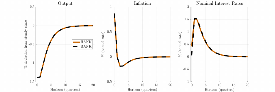
Figure 1: Optimal dual-mandate policy response to a cost-push shock. The RANK model replaces

our general “IS” curve (22) with the simple textbook Euler equation (23). We then calibrate all

parameters as in the headline HANK model (see Section 5.3), with one exception: we set the

elasticity of intertemporal substitution (EIS) to generate the same peak response of output to an

identiﬁed monetary shock as in the HANK model. In practice, the EIS is little changed.

π,ε

· ε

ε, and (ii) the eﬀects of interest rate changes on output and inﬂation, Θ

y,i

and Θ

π,i

will necessarily agree on the optimal interest rate path

∗

We view this irrelevance result as informative because its ingredients are measurable. In

particular, the dynamic causal eﬀects of interest rate changes on aggregate outcomes—that

is, elements of Θ

y,i

and Θ

π,i

—are the estimands of a large empirical literature on monetary

policy shocks (Ramey, 2016). Structural models are often calibrated or estimated to be

consistent with estimates from this literature, which leads them to approximately agree for

the entire matrices Θ

y,i

and Θ

π,i

. The degree to which such quantitative models can disagree

on optimal dual-mandate interest rate paths is thus limited by the empirical evidence.

Quantitative illustration. We close with a quantitative illustration of the analytical

results presented so far. To this end, we study optimal dual-mandate monetary policy in

response to a cost-push shock η

in a calibrated version of our HANK model. Details of the

calibration are postponed until Section 5.3; for purposes of the discussion here, it suﬃces

to note that the model has been parameterized to in particular be consistent with empirical

evidence on the output gap and inﬂation eﬀects of monetary policy shocks. We then contrast

aggregate outcomes in this economy with those in an analogous RANK model, calibrated

similarly to be consistent with empirical policy shock evidence.

Results are displayed in Figure 1. We emphasize the following two main takeaways, both

consistent with our analytical discussion in the earlier parts of this section. First, as shown

in Proposition 1, the output gap and inﬂation paths are exactly the same. The optimal

trade-oﬀ between inﬂation and output is fully governed by the Phillips curve, which itself

is not aﬀected by household inequality. Second, the nominal interest rate path required to

implement the optimal outcome is quite similar across the two models. Intuitively, since by

construction both models match the same evidence on the transmission from interest rate

changes to output and inﬂation, the interest rate movements that achieve the policymaker’s

desired output and inﬂation responses to the shock cannot be too dissimilar.

5 Optimal Ramsey policy

We now turn to the optimal policy problem of a Ramsey planner. Unlike our ad hoc dual-

mandate loss function of Section 4, this planner’s objective is directly aﬀected by household

inequality, reﬂecting a desire to dampen the distributional consequences of aggregate shocks.

Most of our analysis in this section again focuses on optimal monetary policy.

The remainder of the section proceeds in three steps. First, in Section 5.1, we show how

to express the optimal policy problem in our linear-quadratic form. Second, in Section 5.2

we present general analytical results and discuss some instructive analytical special cases.

Finally, in Sections 5.3 and 5.4, we turn to quantitative analysis, leveraging our analytical

“suﬃcient statistics” formulas to connect to empirical evidence to compare our ﬁndings with

those of prior work.

5.1 The optimal policy problem

We consider a conventional Ramsey planner that aggregates utilities of the households pop-

ulating the economy. This section presents a linear-quadratic version of this policy problem.

As is typical in the optimal policy literature (e.g. see the discussion in Giannoni & Wood-

ford, 2002), doing so requires eﬃciency of the steady state. In the representative agent

context, eﬃciency requires that the level of production is optimal. Here we also require that

the planner ﬁnds the steady-state cross-sectional distribution of consumption desirable. Our

optimal policy analysis will therefore capture an insurance motive against ﬂuctuations in

consumption shares, but it will not seek to change the long-run distribution of consumption.

As discussed above, the two interest rate paths would agree exactly if the two models were to agree

on all of Θ

y,i

and Θ

π,i

. Our calibration instead only ensures that peak output and inﬂation responses in

response to a particular, transitory interest rate movement align. This materially limits the extent of—but

does not fully eliminate—possible disagreement in nominal rate paths.

Loss function. To state the loss function, it will prove convenient to describe an individ-

ual’s outcomes in terms of their history of idiosyncratic shocks; that is, we replace c

with

(ζ

where ζ

≡ (ζ

, ζ

it−1

, ζ

it−2

, · · · ) is individual i’s history of idiosyncratic shocks and

(ζ

) ≡ c

is their share of aggregate consumption.

Letting Γ(ζ) denote the (station-

ary) distribution of such histories (with ζ denoting a generic realization of a history), we can

write the social welfare function as

∞

t=0

ϕ(ζ)

(ω

(ζ)c

)

1−γ

− 1

1 − γ

− ν (`

)

dΓ(ζ), (32)

where ϕ(ζ) is a Pareto weight on the utility of households with history ζ.

In keeping with optimal (monetary) policy analysis in standard representative-agent en-

vironments (Woodford, 2003), our objective is to evaluate the social welfare function (32)

to second order. To this end, a ﬁrst-order approximation to aggregate equilibrium dynamics

suﬃces only if the expansion point (i.e., the deterministic steady state) is eﬃcient. Without

household heterogeneity, a simple production subsidy is suﬃcient to ensure this. With house-

hold heterogeneity, however, we now also require the consumption shares of all households

to be optimal. In principle there are two ways of ensuring this: either the steady-state ﬁscal

tax-and-transfer system achieves the optimal level of insurance given the planner weights

ϕ(•), or the planner weights are set residually so that the implied steady-state distribution

of consumption given a tax-and-transfer system is optimal. We adopt the second approach,

following the inverse optimal taxation literature (e.g. Heathcote & Tsujiyama, 2021). Our

preference for this approach reﬂects the overarching focus of this paper: we ask how cyclical

policy tools should be manipulated to respond to cyclical changes in inequality, leaving the

long-run steady state outside of the purview of our analysis.

Appendix D.3 presents our assumptions on the production subsidy and policymaker pref-

erence weights that ensure eﬃciency of the deterministic steady state. Given those assump-

tions, a second-order approximation of (32) around the eﬃcient steady state then gives the

following characterization of the policymaker loss function.

Proposition 2. To second order, the social welfare function V

is proportional to −L

given by

≡

∞

t=0



bπ

˜κ

¯η

+ λ

bω

(ζ)

¯ω(ζ)

dΓ(ζ)



, (33)

Note that this is without loss of generality, as individuals in our model are ex ante identical, so their

outcomes only diﬀer due to diﬀerent histories of shocks.

where bω

(ζ) = ω

(ζ) − ¯ω(ζ) and ¯ω(ζ) is the steady-state consumption share of an individual

with history ζ and ˜κ and λ

are composite parameters deﬁned in Appendix D.3.

Note that, in the representative-agent analogue of our economy (as discussed in Sec-

tion 3.5), the loss function would feature the same ﬁrst two terms, as already well-known

from prior work (Woodford, 2003).

Our analysis reveals that household heterogeneity adds

a third, inequality-related term, with the planner wishing to stabilize the consumption shares

of everyone in the economy.

How does the inequality term in (33) ﬁt into the linear quadratic framework in Section 2?

Moving to a sequence-space formulation, we can write the loss as

= λ

π + λ

y +

ω(ζ)

ω(ζ)dΓ(ζ), (34)

where λ

= 1, λ

˜κ

¯η

, and λ

≡ λ

/¯ω(ζ). The consumption share for each idiosyncratic

household history thus emerges as a separate target variable for the policymaker. We will

discuss our approach to computation of (34) later in this section.

Constraints. The constraints of the optimal policy problem characterize the evolution

of policymaker targets—π, y, and the consumption shares ω(ζ)—as a function of exogenous

shocks and policy choices. As we discussed in Section 4.1, the evolution of aggregate output

and inﬂation are governed by the Phillips curve (21) and the IS curve (22). It then remains

to describe the evolution of the inequality term in (33). In Appendix C.2, we establish that,

to ﬁrst order, we can write the consumption share for a household with speciﬁc history ζ as

ω(ζ) = Ω

ω(ζ),x

x, ∀ζ (35)

where x

x = (y

y, r

r,τ

,τ

m, π

, q

) stacks the prices and shocks that aﬀect the household de-

cision problem, and the maps Ω

ω(ζ),x

give the derivatives of consumption shares with respect

to these aggregate variables. The intuition for (35) is the same as that for the aggregate

consumption function—an individual household’s consumption, given their history of id-

iosyncratic shocks, evolves over time as a function of the aggregate inputs to the household

When δ = 0 (so there is no investment spending) the composite term ˜κ reduces to κ, and so the ﬁrst

two terms in the loss function are exactly the same as the familiar ones from the literature.

Note that, technically, (34) does not immediately ﬁt into our framework in Section 2.1 since the objective

here features an integral (rather than a simple sum). Our approach to computation will consider an equivalent

formulation of the problem with ﬁnitely many policy targets.

consumption-savings problem. By the proof of Lemma 1, we can obtain these inputs as a

function of exogenous shocks, policies, and aggregate output and inﬂation paths.

For future reference it will be useful to note that, again following McKay & Wolf (2023),

we can alternatively re-write this constraint in impulse response space, solving out the de-

pendence of consumption shares on endogenous aggregates:

ω(ζ) = Θ

ω(ζ),i

i + Θ

ω(ζ),x

+ Θ

ω(ζ),η

η + Θ

ω(ζ),m

m. ∀ζ (36)

Summary & computational details. The Ramsey planner chooses paths of the two

available policy instruments—nominal interest rates i

i and the exogenous component of trans-

fers τ

—to minimize the derived loss function L

subject to the same two constraints as

before, (25) and (26), as well as the evolution of the inequality term, (36).

To computationally evaluate the more complicated loss function (34) and the associated

constraints, we show in Appendix C.2 that the Ramsey loss can be re-written as

π +

˜κ

¯η

y + λ

x (37)

where Q is a linear map, deﬁned in Appendix C.2.

The alternative formulation in (37)

reﬂects the simple insight that it is always possible to re-write the loss coming from cross-

sectional inequality as a function of the (small number of) inputs to the consumption-savings

problem—income, interest rates, asset prices, taxes, and shocks. With the re-written loss

function (37), the relevant constraints are then simply the equilibrium dynamics of x

x. Com-

putation is thus again straightforward: Appendix C.2 discusses how to recover the map Q,

while the coeﬃcient matrices for all constraints are again immediate from standard sequence-

space solution output, exactly as in the dual-mandate problem considered before. To summa-

rize, relative to solving a HANK model given a policy rule, the only additional computational

work needed to solve a Ramsey optimal policy problem is the one-time computation of the

auxiliary linear map Q.

5.2 Optimal policy rules

Having expressed the optimal Ramsey problem in linear-quadratic form, we can now leverage

the results of Section 2 to provide a general characterization of optimal Ramsey policy rules.

We note that the linear map Q in (37) is in general not diagonal. Thus Appendix C.2 also extends the

results from Section 2 to the case with such interaction terms.

The optimal Ramsey monetary policy rule is given as

π,i

π +

˜κ

¯η

y,i

y +

ω(ζ),i

ω(ζ)dΓ(ζ) = 0

0, (38)

where as before the matrices Θ

•,i

collect the dynamic causal eﬀects of interest rate move-

ments on the various policymaker targets—our “suﬃcient statistics” for optimal policy. In

particular, we see that the ﬁrst two terms in (38) are identical to the optimal dual-mandate

rule (29), just now with weights derived from policymaker preferences (rather than exoge-

nously assumed). The novel third term—which reﬂects the planner’s distributional insurance

concerns—collects the causal eﬀects of interest rate movements on consumption shares. Pro-

ceeding analogously for stimulus checks we ﬁnd the optimal rule

π,τ

π +

˜κ

¯η

y,τ

y +

ω(ζ),τ

ω(ζ)dΓ(ζ) = 0

0, (39)

As discussed in Wolf (2021) and also brieﬂy in Section 4.2, nominal interest rate and stimulus

check policy in our environment can implement exactly the same output-inﬂation allocations,

so the ﬁrst two terms in (38) and (39) will reﬂect identical aggregate stabilization objectives.

The distributional terms Θ

ω(ζ),i

and Θ

ω(ζ),τ

, on the other hand, will generally diﬀer, thereby

opening the door for interest rate and stimulus check policies to be useful complementary

tools for aggregate stabilization. We will return to this observation in Section 5.4. Overall,

(38) and (39) fully characterize joint optimal monetary-ﬁscal policy.

The key takeaway from the characterizations in (38) and (39) is that optimal policy rules

in the general Ramsey problem deviate from the dual-mandate rules discussed in Section 4

if and only if the policy instruments aﬀect cross-sectional consumption inequality. On the

one hand, if monetary policy is distributionally neutral—as is for example the case in the

environment of Werning (2015) (see Appendix A.2 for details)—then household inequality

does not aﬀect the optimal rule: setting Θ

ω(ζ),i

= 0

0 and simplifying (38), we ﬁnd that the

optimal Ramsey rule continues to take a standard dual-mandate form

bπ

¯η

(by

− by

t−1

) = 0, ∀t = 0, 1, . . . (40)

Bilbiie (2021) makes an analogous argument in a two-agent context, showing that, if monetary policy

does not redistribute between spenders and savers, then the optimal policy rule is not aﬀected by inequality

concerns. Our analysis reveals that the conditions underlying Werning’s aggregation result are precisely

enough to extend this insight to our heterogeneous-agent setting.

In this case, monetary policy optimally focuses on aggregate objectives while ﬁscal policy

takes sole responsibility for all distributional considerations. On the other hand, if interest

rate cuts are strongly progressive (as is the case in Bhandari et al., 2021; D´avila & Schaab,

2022), then the concerns about inequality as embedded in the policymaker objective (33)

may materially change optimal monetary policy conduct, with insurance concerns swamping

the usual price and output stabilization motives. This discussion suggests the way forward:

to provide a convincing answer to the question of whether household inequality aﬀects the

optimal Ramsey policy, researchers should consider structural models that agree with empir-

ical evidence on the distributional incidence of policy, as embedded in our suﬃcient statistics

formulas in (38) - (39). The next subsection discusses how we do so.

5.3 Calibration

We seek to calibrate our structural model to deliver empirically realistic distributional eﬀects

of monetary and ﬁscal stabilization policy. In particular, as revealed by our formulas in (38)

and (39), what ultimately matters are the eﬀects of policy on consumption inequality. Some

prior empirical work has tried to directly estimate those causal eﬀects. The results so far,

however, are not conclusive: while Holm et al. (2021) ﬁnd that expansionary monetary policy

has moderately pronounced U-shaped eﬀects on consumption in the wealth cross-section (in

Norway), Coibion et al. (2017) report declines in consumption inequality, and Chang &

Schorfheide (2022) conclude that inequality actually even increases somewhat (both in the

U.S.). In addition to cross-country institutional diﬀerences, this lack of consensus is likely

to reﬂect the lack of high-quality, high-frequency consumption data.

In light of these challenges with direct measurement, we instead proceed as follows.

We calibrate the model to empirical evidence on how monetary policy aﬀects the various

components of household income—for which there is much more consensus as we describe

below. We then rely on the structure of our model’s consumption-savings problem to map

these eﬀects on income into eﬀects on consumption—the suﬃcient statistics that ultimately

enter our optimal policy formulas (38) and (39). The remainder of this section implements

this approach by proceeding in three steps. First, we review the empirical evidence on how

monetary policy aﬀects income and wealth in the cross-section of households. Second, we

calibrate our model so that it captures those channels of redistribution as well as possible.

And third, we use the model to infer the total eﬀects of monetary policy on the consumption

distribution, bringing together the eﬀects from the various channels.

The distributional effects of monetary policy. We begin with a brief review of

the most important transmission channels from monetary policy to household balance sheets.

a) Labor income. There is extensive evidence that those with less education, low past earn-

ings, and racial minorities tend to be more exposed to cyclical ﬂuctuations in labor market

conditions (e.g. Okun, 1973; Hoynes, 2000; Guvenen et al., 2014; Patterson, 2022). Turn-

ing to monetary policy more speciﬁcally, Guvenen et al. (2014) study earnings dynamics

in the 1979–1983 recession—a contraction that was arguably caused by a large monetary

intervention. They ﬁnd that individuals with low previous earnings also suﬀered the

largest earnings losses. Several recent studies combine identiﬁed monetary policy shocks

with European administrative data and arrive at very similar conclusions (Andersen et al.,

2021; Amberg et al., 2021; Holm et al., 2021).

In addition to the distribution of labor income, there is also the question of how strongly

total labor income responds to monetary policy. As is well-known, in textbook sticky-

price, ﬂexible-wage models, expansionary monetary policy sharply increases labor income,

thus giving monetary policy power to redistribute between workers and ﬁrm owners.

Empirically, on the other hand, studies have found that expansionary policy leads to a

modest rise in real wages and proﬁts.

Our model, due to our assumptions on the division

of monopoly proﬁts between workers and ﬁrm owners, implies that total compensation

and returns to capital move one-for-one with output, consistent with the evidence.

b) Asset prices. Expansionary monetary policy raises the value of long-duration assets and

leads to considerable capital gains for the owners of those assets. For example, Bauer &

Swanson (2022) estimate that a 100 basis point reduction in short-term nominal interest

rates increases the S&P 500 stock market index by about ﬁve percentage points. As the

distribution of wealth is concentrated, these capital gains are very unequally distributed

across the population. Andersen et al. (2021) leverage administrative household-level data

from Denmark to quantify this distributional gradient. They ﬁnd that, in response to a

one percentage point decrease in the policy rate, asset values increase by around 70 per

cent of total annual disposable household income at the top of the income distribution,

and around 30 per cent at the median.

See the summary in Christiano et al. (1999). Relatedly, Cantore et al. (2021) ﬁnd that expansionary

policy leads to a decrease in the labor share—opposite the response in textbook New Keynesian models.

Of course, while long-duration real assets increase in value following an expansionary monetary shock,

so too do the values of long-duration liabilities. In particular, the future consumption plans of households

c) Nominal wealth redistribution. Surprise inﬂation will lower the real value of nominal po-

sitions. Doepke & Schneider (2006) report that wealthy households have about 10-15%

of their net worth in nominal positions, while young middle-class households have consid-

erable nominal liabilities in the form of mortgages. The magnitude of the redistribution

that occurs through this channel of course depends on the strength of the inﬂation re-

sponse to monetary policy. Many empirical studies point to a relatively ﬂat Phillips curve

(see e.g. the review in Mavroeidis et al., 2014), thus implying relatively small inﬂation

responses to changes in policy. However, we note that the resulting distributional eﬀects

can be permanent if monetary policy allows permanent changes in the price level.

d) Net interest income. Expansionary policy lowers interest rates, thus leading to lower

debt service payments for debtor households and to lower interest income for creditor

households. This channel beneﬁts middle-class households that own a home with a large

mortgage relative to their net worth (see Cloyne et al., 2020; Wong, 2021).

Model calibration. We calibrate our model to capture the just-summarized channels

of monetary policy propagation to consumption inequality.

• Income process. Since many of the distributional eﬀects of monetary policy involve

changes in asset values, it is important that the model generates a concentrated dis-

tribution of wealth, mirroring the data. Since standard incomplete-markets models of

the consumption-savings decision struggle to generate suﬃciently concentrated wealth

holdings in the top tail of the distribution, we follow Castaneda et al. (2003), Boar

& Midrigan (2020), and Greenwald et al. (2021) in specifying an income process with

superstar earners, allowing us to generate a realistic concentration of wealth.

We assume that the underlying household income state, ζ

, follows a two-component

process, with households being either regular workers or high earners. The function Φ

that maps ζ

to labor productivity e

is parameterized as

log e

= log [(1 − α)y

] + log (ζ

) (1 + m

+ χ log y

) + log ¯e

, (41)

where χ controls the sensitivity of income dispersion to the aggregate business cycle,

with a negative χ implying that low-ζ households are more exposed to the cycle, and

become more costly as real interest rates fall. The theoretical ideal to measure the net exposure to interest

rates, accounting for the diﬀerence between asset income and planned consumption (see e.g. the discussion

in Auclert, 2019). Our model will embed these eﬀects on the present value of consumption liabilities.

Wealth Income

Data Model Data Model

Top 1% 37 27 17 20

Top 5% 65 66 32 32

Top 10% 76 82 43 44

Top 25% 91 96 64 60

Top 50% 99 101 84 77

Table 1: Shares (%) of wealth and income concentrated in the top x% of the distribution. Data

are from the 2019 Survey of Consumer Finance.

¯e

is a normalization constant ensuring that

di = (1 − α)y

at all dates.

For

regular workers, the state log ζ

follows an AR(1) process. High-earning households

instead can receive one of two (high) levels of earnings. There are thus six parameters

associated with the high-earnings states: the probability of becoming a high earner

of either kind, the earnings level associated with each state, and the probabilities of

transitioning back to being a regular worker.

To estimate the full income process we extend the estimation procedure of Guvenen

et al. (2022). Those authors propose a rich parametric income process that allows for

diﬀerential exposure to aggregate business-cycle conditions, and then estimate it using

a variety of moments taken from the Social Security Administration data. This strategy

pins down χ in (41) using data on the diﬀerential impact of business-cycle episodes

across the income distribution. We extend their procedure by also targeting moments

of the wealth and income distribution, as reported in Table 1. Further details on the

calibration of the income process and its parameters are presented in Appendix B.1.

• Asset structure. In the model, households have positions in capital, short-term bonds,

and long-term bonds. We need to calibrate the total supply of each asset class and then

how these assets are distributed in steady state. The steady state portfolios determine

the distribution of capital gains at t = 0, when the economy is subjected to shocks.

We use data on the balance sheets of U.S. households from the Financial Accounts and

the 2019 SCF to impute the holdings of particular asset classes across the household

Regular workers share a common value of χ while high earners have χ = 0.

To reduce the number of parameters, we assume that there are no transitions between the high-earning

states and that upon exit the individual receives a random draw from the unconditional distribution of

regular worker ζ’s.

Holdings by net worth group

Line Category Total

Top Next Next Bottom

1% 9% 40% 50%

1 Real estate and durables 167 24 48 72 23

2 Equity and mutual funds 191 101 66 23 2

3 Currency, deposits, and similar 60 16 23 19 2

4 Govt. and corp. bonds and similar 29 10 11 7 1

5 Pension assets 131 6 63 58 4

6 Mortgage liabilities 49 2 12 24 11

7 Consumer credit and loans 24 1 2 8 12

8 Net worth excluding pension assets 374 147 135 89 4

9 Capital 419 157 135 101 25

10 Short-term bonds -12 1 7 -3 -16

11 Long-term bonds -33 -11 -8 -9 -5

12 Total 374 147 135 89 4

Table 2: Assets and liabilities in percent of GDP with decomposition by net-worth. Lines 1-8

report the observed asset and liability categories from the Distributional Financial Accounts. Lines

9-12 map these assets and liabilities into their model counterparts.

distribution of net worth. The top panel of Table 2 reports data on asset holdings in

coarse net worth bins, taken from the Distributional Financial Accounts (DFAs).

important takeaway from Table 2 is that pension assets represent 22% of total house-

hold assets. Of these pension assets, 61% are deﬁned beneﬁt entitlements. Given that

we do not explicitly model pensions we must make a choice about how to incorporate

these assets into our calibration. As households are quite insulated from the returns on

these pension assets, we choose to incorporate the pension funds on to the government

balance sheet. The returns on these pension assets are then gradually paid out to

households through adjustments in taxes.

The next step is to map the observed asset categories into the corresponding asset

classes in the model. We treat corporate and non-corporate equity as levered claims

on capital, so each dollar of equity represents $1.32 dollars of capital and a $0.32 debt

position. This leverage ratio reﬂects the ratio of debt to assets in the non-ﬁnancial

business sector. Based on the results in Greenwood et al. (2010) we assume that 62%

Our imputation procedure yields similar results to the DFAs, but we use the SCF to create portfolios

that are smooth functions of net worth as opposed to the coarse bins shown in Table 2.

of this debt is long-term debt. We set the duration of the long-term bond in our model

to 10 years, in line with results for corporate bonds in Guedes & Opler (1996). Next,

we treat mortgages as a 50-50 split of short-term and long-term debt. Even though

many mortgages are 30-year loans, the duration of these loans is much shorter due

to amortization and prepayment (e.g., Greenwald et al., 2021, report a duration of

approximately 5 years). We treat consumer credit as short-term debt. Overall our

choices lead to a capital-output ratio of 4.19, as shown in Table 2. In total, households

have debts of 12% of GDP in short-term bonds and 33% of GDP in long-term bonds.

We set the capital share to α = 0.36 and the depreciation rate to δ = 0.01, allowing

us to match a 17% investment rate (the average observed from 1984 to 2019). These

values imply a steady state annual interest rate of 4.5%. Lastly, we set the borrowing

limit—which restricts net worth and not gross positions—to −0.27 times steady state

average income. This value matches the 5th percentile of net worth in our SCF data.

• Fiscal system. The U.S. ﬁscal tax-and-transfer system is reasonably well-approximated

by a uniform baseline lump-sum transfer coupled with a constant marginal tax rate (see

Kaplan et al., 2018). Data on post-government and pre-government income from the

Congressional Budget Oﬃce (2019) imply a steady state transfer of 0.17 times average

income, pinning down the ratio ¯τ

/¯y in our model.

The speed of ﬁscal adjustment is

controlled by σ

, which we set equal to σ

, implying very gradual ﬁscal feedback.

• Other parameters. We set the Frisch elasticity to one, and the elasticity of substitution

between labor varieties to six, based on Basu & Fernald (1997). Finally, we set the

coeﬃcient of relative risk aversion γ and the slope of the Phillips curve κ to match

the peak responses of output and inﬂation to an empirically identiﬁed monetary policy

shock, ensuring that our model is not just consistent with distributional incidence, but

also with overall level responses. Again, the details for this internal calibration are

provided in Appendix B.1.

As households (excluding pension funds) collectively have negative credit positions, the pension funds

will lend to the households and to the government. As we consolidate the pension funds and government

in our model, it is thus as if the government is lending to the households. See Appendix B.2 for further

description of how we use the SCF to impute asset positions as smooth functions of household net worth.

We exclude Medicaid and CHIP beneﬁts from the after-tax income. We then regress after-tax incomes

on before-tax incomes for the ﬁrst four quintiles of the income distribution. The intercept of this regression

gives us the steady state transfer.

We have found that the results are robust to the choice of σ

as long as it takes a low value. Empirically,

changes in public debt are highly persistent, thus implying a low value of σ

Parameter Description Value Calibration target

Households

{ζ

} Income risk process – See text

χ Income exposure -2.0 Het. earnings cyclicality

γ Relative risk aversion 1.2 Monetary shock eﬀects

φ Frisch elasticity 1 Standard

β Discount factor 0.984 Asset market clearing

Firms

κ Phillips curve slope 0.022 Monetary shock eﬀects

¯η Labor Substitutability 6 Basu & Fernald (1997)

Asset Structure

α Capital share 0.36 Standard

δ Depreciation rate 0.01 Investment rate

a/¯y Borrowing limit −0.27 Fifth percentile of net worth

Long-term bond duration 0.025 Guedes & Opler (1996)

Government

Labor tax rate 0.23 Steady-state budget balance

¯τ

¯y

Transfer share 0.17 After-tax vs. before-tax income

Tax-debt responsiveness = σ

See text

Table 3: Calibration of our quantitative HANK model. The model period is one quarter.

We summarize all parameter values in Table 3.

Consumption responses. Having calibrated our model to be consistent with the most

salient transmission channels of monetary policy to households, we now use the structural

model to map these income responses into the suﬃcient statistics that ultimately enter our

optimal policy rules—the eﬀects of monetary policy on consumption inequality.

Figure 2 shows the model-implied impact change in consumption across the wealth distri-

bution following a transitory, expansionary monetary policy shock. Since histories ζ map into

diﬀerences in income and wealth, we note that this ﬁgure is directly informative about the

ω(ζ),i

’s that enter our optimal policy rules. Our main ﬁnding is that households across the

wealth distribution increase their consumption relatively uniformly, implying small eﬀects

on consumption shares—that is, causal eﬀects Θ

ω(ζ),i

that are quite close to zero.

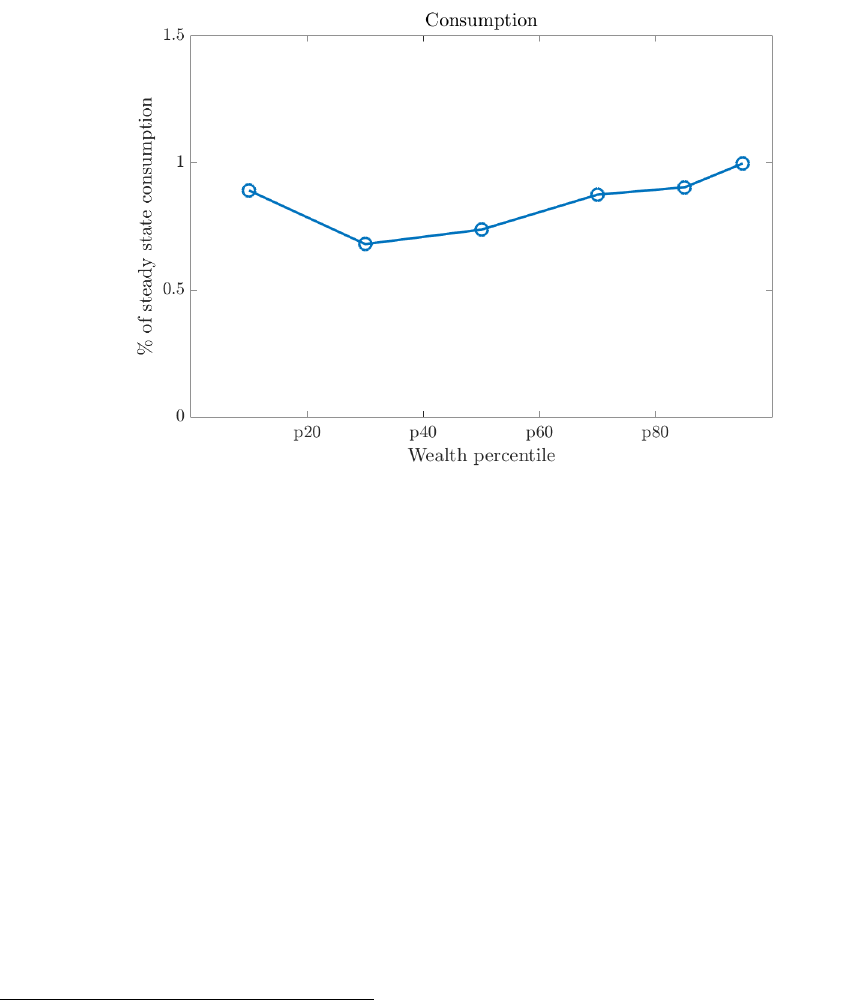
Figure 2: Initial response of consumption to an expansionary monetary policy shock across the

distribution of wealth. We simulate the shock we estimate empirically in Appendix B.1.

What explains these rather evenly distributed eﬀects of policy stimulus? On the one end

of the spectrum, low-wealth households tend to also have rather low incomes, their labor

earnings are more exposed to aggregate income, and they are often borrowing-constrained

and so tend to have high marginal propensities to consume (MPCs). As a result, changes

in labor earnings pass through strongly into consumption. Households with a moderate

amount of wealth instead tend to have substantial real estate and mortgage positions (see

the Next 40% column in Table 2), and also relatively moderate MPCs. Finally, high-wealth

households beneﬁt from increases in asset values. While these capital gains are very large, the

pass-through to consumption is relatively weak, given the rather low model-implied MPCs

at the top end of the wealth distribution.

Putting all of the pieces together, we arrive at

the relatively uniform eﬀects shown in Figure 2.

Note that the earnings of the lowest-wealth group increase by 0.5% of their steady-state income, while

the capital gains of the highest-wealth group amount to more than 20% of steady-state income. The model

is thus fully consistent with the empirical results of Andersen et al. (2021) and Bartscher et al. (2021), who

emphasize that capital gains eﬀects are large relative to labor income eﬀects. While the implications for

short-run consumption are more equal, high-wealth consumption does remain elevated for longer. These

dynamic eﬀects are not visible in Figure 2, but they are incorporated into our analysis of optimal policy.

5.4 Applications

We now use the calibrated model as a laboratory to explore optimal Ramsey policy in two

scenarios. As our ﬁrst application, we consider an aggregate shock with strong distributional

consequences, depressing consumption of the poor relative to that of the rich, akin to the

Covid-19 recession. Second, we return to the inﬂationary cost-push shock from Section 4.3—

a shock that has received much attention in the classic RANK literature as well as the recent

HANK literature (e.g., Bhandari et al., 2021; Acharya et al., 2022). We will use this second

application and the comparison with prior work to in particular highlight the usefulness of

our suﬃcient statistics approach to optimal policy rule characterization.

Distributional shock. Our ﬁrst shock is an innovation to m

, the exogenous driver of

income dispersion in (41). This shock redistributes labor income from low-income to high-

income households, thus depressing aggregate demand: precautionary savings increase due

to the increase in risk, and so spending falls as income is redistributed towards lower-MPC

households. We study three optimal policy responses to this demand shock: monetary policy

for a dual mandate policymaker; monetary policy for a Ramsey planner; and ﬁnally joint

monetary-ﬁscal policy for a Ramsey planner. Results are reported in Figure 3.

We begin with the optimal dual mandate policy response, displayed as the grey lines

in Figure 3. As aggregate demand falls, the dual-mandate central banker cuts nominal

interest rates to perfectly stabilize output and inﬂation (the classic “divine coincidence”).

The bottom panel shows how the consumption distribution changes on impact of the shock:

the shock itself redistributes from low-income to high-income households, and monetary

policy—precisely because of how we calibrated the model—does very little to oﬀset that.

We then consider the optimal Ramsey monetary policy that also considers distributional

objectives, depicted as the orange dashed lines in Figure 3. Our headline ﬁnding here is that

the optimal policy response is very similar to the dual-mandate policy, with nominal interest

rates now cut somewhat more on impact of the shock but then very closely following the

dual mandate policy. As a result, aggregate output and inﬂation continue to be stabilized

almost perfectly, and the response of the consumption distribution hardly diﬀers from the

dual-mandate outcome. The intuition is as follows. The original shock m

has a strong

distributional tilt, with low-income households losing the most. The Ramsey planner would

like to lean against this redistribution and stabilize consumption shares. Monetary policy,

however, is a rather blunt tool: if the planner were to cut rates by enough to stabilize

consumption at the bottom of the distribution, then consumption of richer households and

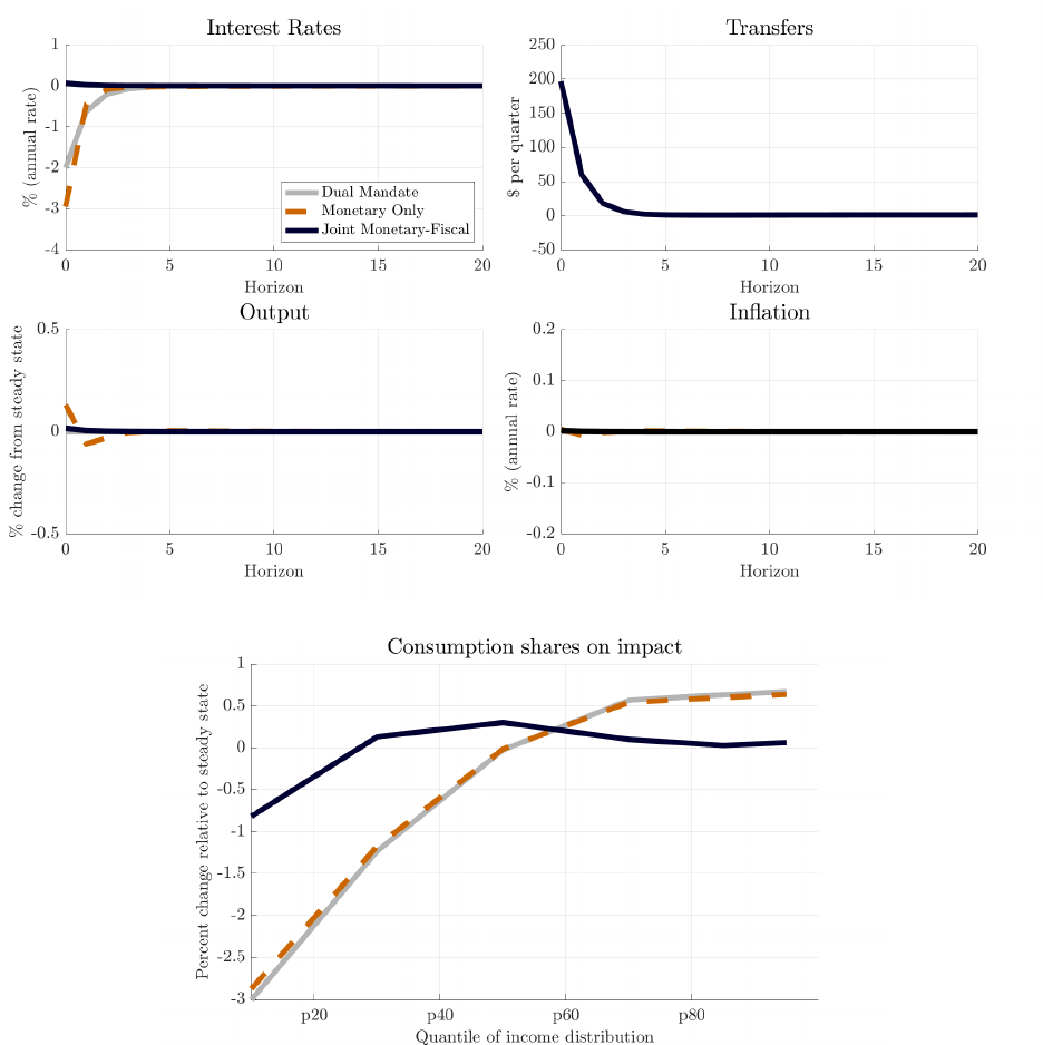
Figure 3: Optimal policy response to an income distribution shock m

. The ﬁgure shows the

results from three policy rules: optimal monetary policy for a dual-mandate policymaker (Dual

Mandate), optimal monetary policy for a Ramsey planner that is constrained not to use lump-sum

transfers (Monetary Only), and optimal policy for a Ramsey planner that can use both tools (Joint

Monetary-Fiscal). Transfers are expressed in units of dollars, using the conversion that steady state

per capita GDP is $60,000.

so aggregate output and inﬂation would overshoot signiﬁcantly—an immediate implication

of the ﬂat distributional eﬀects of monetary interventions shown in Figure 2. We provide a

visual illustration of this point in Appendix Figure B.4: increasing the size of the interest

rate cut to stabilize the consumption of households with low income and low wealth comes

at the cost of over-stimulating the consumption of other households (and thus aggregate

output and inﬂation).

Finally we turn to the optimal joint monetary-ﬁscal Ramsey policy, with a planner using

both interest rate policy and stimulus checks to pursue her aggregate and distributional

objectives. Results are displayed as the dark blue lines in Figure 3. Compared to monetary

policy, ﬁscal stimulus payments are much more progressive, with consumption of low-income

and low-wealth households responding signiﬁcantly more than that of high-income, high-

wealth households (see Wolf (2021) or Appendix Figure B.3). Intuitively, this reﬂects both

diﬀerences in MPCs as well as diﬀerences in income levels, with any given dollar amount of

stimulus checks amounting to a much larger fraction of income at the bottom of the income

distribution. As a result, ﬁscal stimulus payments are particularly well-suited as a tool to

address shocks that diﬀerently aﬀect low-income and high-income households. The results

depicted in Figure 3 are consistent with this intuition: in response to the distributional

shock m

, the Ramsey planner can use checks to almost perfectly stabilize aggregate output,

inﬂation, and consumption inequality. Since stimulus payments both compress inequality

and stimulate aggregate demand, there is little need for the monetary authority to intervene,

with nominal interest rates now responding very little.

Overall, our analysis of optimal Ramsey policy responses to the distributional demand

shock m

suggests two broad lessons for optimal cyclical policy design. First, recall from our

prior analysis that a monetary policymaker has an incentive to deviate from the prescrip-

tions of dual mandate policy only if monetary policy can help her to oﬀset the distributional

incidence of the underlying business-cycle shock. With empirical evidence suggesting a rel-

atively uniform distributional incidence of monetary interventions, it follows that monetary

policy is in general rather ill-suited to attain distributional objectives. In particular, sta-

bilizing consumption at the bottom of the distribution may require signiﬁcant departures

from dual-mandate objectives; if the Ramsey planner is unwilling to accept these departures

(as was the case in our example), then optimal policy will tend to stay close to the dual-

mandate benchmark, as seen here. Second, ﬁscal stimulus payments and nominal interest

rate policy can be highly complementary policy tools. They are likely to have very diﬀerent

cross-sectional incidence proﬁles (see Figure 2 and Figure B.3), and so the optimal mix of

Figure 4: Optimal policy response to an inﬂationary cost-push shock. The ﬁgure shows optimal

monetary policy for a planner whose objective is to stabilize output and inﬂation (Dual Mandate)

and for a Ramsey planner (Monetary Ramsey).

monetary and ﬁscal policy as a stabilization tool will depend on the distributional incidence

of the shocks hitting the economy.

Cost-push shock. Our second shock is a classic cost-push shock η

, as already considered

in our dual-mandate application in Section 4.3. In our model, this cost-push shock introduces

a wedge in the aggregate Phillips curve, thus giving an output-inﬂation trade-oﬀ. Under our

assumptions on the incidence of ﬁrm proﬁts, however, this shock does not by itself have

strong distributional implications. For our analysis we restrict attention to monetary policy

alone, comparing only the optimal dual-mandate and Ramsey monetary policy responses.

Results are displayed in Figure 4. We ﬁnd that the Ramsey policy is nearly identical to the

dual-mandate policy. Intuitively, neither the shock nor the monetary policy response has

strong distributional eﬀects, and so there is little reason to deviate from the dual mandate

policy. Furthermore, by the logic discussed above, this result is unlikely to change materially

even if the cost-push did have meaningful distributional eﬀects, simply because monetary

policy would still be ill-suited to oﬀset those.

Our ﬁndings contrast with recent arguments made in Bhandari et al. (2021), who con-

clude that distributional considerations may lead to substantial changes in optimal policy

conduct—changing the signs of impulse response functions and the order of magnitude of

inﬂation volatility. Our analysis diﬀers from theirs both methodologically and due to the as-

sumptions on the economic environment. To demonstrate that the diﬀerence in conclusions

is driven to a considerable extent by the economic assumptions, Appendix B.4 repeats our

analysis of the cost-push shock in an alternative model environment that is more similar to

that in Bhandari et al.. In particular, for this alternative environment, we assume that (i) all

monopoly proﬁts are distributed to wealthy ﬁrm owners and (ii) there are no other types of

long-duration assets (i.e., the model omits capital and housing-related assets and liabilities).

This change in the model environment has two implications. First, cost-push shocks now

have strong distributional eﬀects: they increase markups, decrease real wages, and increase

the proﬁts ﬂowing to a concentrated group of ﬁrm owners. Second, expansionary monetary

policy is also redistributive, but in the other direction—it reduces markups, raises real wages,

and reduces proﬁts. In light of our previous discussion it is thus unsurprising that we ﬁnd an

optimal Ramsey monetary policy closely echoing the conclusions of Bhandari et al.: while

a dual mandate policymaker hikes interest rates following a cost-push shock, the Ramsey

planner instead sharply lowers them to reduce cross-sectional inequality.

6 Conclusion

Should household inequality aﬀect the conduct of cyclical stabilization policy? The analysis

in this paper suggests the following three main takeaways.

First, for central banks that target standard macroeconomic aggregates (e.g., a traditional

“dual mandate”), household inequality—at least as typically modeled in the burgeoning

HANK literature—is likely to only have rather moderate eﬀects. Analytically, we have

given conditions under which the optimal forecast target criterion of a dual mandate central

banker is unaﬀected by household inequality, implying that output and inﬂation outcomes

in response to any shock will be exactly as in analogous representative-agent environments.

Empirically, a long literature already estimates the causal eﬀects of interest rate changes

on output and inﬂation. Models that are consistent with this evidence will yield similar

predictions for the paths of nominal rates necessary to implement a given output and inﬂation

target—irrespective of whether the model features household inequality or not.

Second, the extent to which distributional objectives shape optimal Ramsey monetary

policy depends crucially on the causal eﬀects of interest rate changes on consumption inequal-

ity. According to our analysis, monetary policy has relatively even eﬀects on consumption

across households. Interest rate policy is thus not a particularly sharp tool to deal with

shocks that disproportionately aﬀect the poor, at least not without substantial costs in

terms of aggregate stabilization.

Third, ﬁscal stimulus checks—an alternative tool of stabilization policy, used increasingly

frequently in recent decades—promise to be more useful for distributional purposes. Such

stimulus checks achieve aggregate stabilization through insurance at the bottom, thus making

them well suited to address cyclical ﬂuctuations that mostly aﬀect poor households.

References

Acharya, S., Challe, E., & Dogra, K. (2022). Optimal monetary policy according to HANK.

Forthcoming American Economic Review.

Alves, F., Kaplan, G., Moll, B., & Violante, G. L. (2020). A further look at the propagation of

monetary policy shocks in hank. Journal of Money, Credit and Banking, 52 (S2), 521–559.

Amberg, N., Jansson, T., Klein, M., & Rogantini Picco, A. (2021). Five facts about the

distributional income eﬀects of monetary policy. CESifo Working Paper.

Andersen, A. L., Johannesen, N., Jørgensen, M., & Peydr´o, J.-L. (2021). Monetary policy

and inequality. Working Paper.

Auclert, A. (2019). Monetary policy and the redistribution channel. American Economic

Review, 109 (6), 2333–67.

Auclert, A., Bard´oczy, B., & Rognlie, M. (2020). Mpcs, mpes and multipliers: A trilemma

for new keynesian models. Technical report, National Bureau of Economic Research.

Auclert, A., Bard´oczy, B., Rognlie, M., & Straub, L. (2021). Using the sequence-space

jacobian to solve and estimate heterogeneous-agent models. Econometrica, 89 (5), 2375–

2408.

Auclert, A. & Rognlie, M. (2018). Inequality and aggregate demand. Technical report,

National Bureau of Economic Research.

Auclert, A., Rognlie, M., Souchier, M., & Straub, L. (2021). Exchange rates and monetary

policy with heterogeneous agents: Sizing up the real income channel. Technical report,

National Bureau of Economic Research.

Auclert, A., Rognlie, M., & Straub, L. (2018). The intertemporal keynesian cross. Technical

report, National Bureau of Economic Research.

Bartscher, A. K., Kuhn, M., Schularick, M., & Wachtel, P. (2021). Monetary policy and

racial inequality. CEPR Discussion Paper No. DP15734.

Basu, S. & Fernald, J. G. (1997). Returns to scale in us production: Estimates and implica-

tions. Journal of political economy, 105 (2), 249–283.

Bauer, M. D. & Swanson, E. T. (2022). A reassessment of monetary policy surprises and

high-frequency identiﬁcation. National Bureau of Economic Research Working Paper.

Benigno, P. & Woodford, M. (2012). Linear-quadratic approximation of optimal policy

problems. Journal of Economic Theory, 147 (1), 1–42.

Bernanke, B. (2015). Remarks at Brookings Institution: Objections to Federal Reserve

Accountability Bill.

Bhandari, A., Evans, D., Golosov, M., & Sargent, T. J. (2021). Inequality, business cycles,

and monetary-ﬁscal policy. Econometrica, 89 (6), 2559–2599.

Bilbiie, F. O. (2021). Monetary policy and heterogeneity: An analytical framework. Working

Paper.

Bilbiie, F. O., Monacelli, T., & Perotti, R. (2021). Stabilization vs. redistribution: the

optimal monetary-ﬁscal mix. CEPR Discussion Paper No. DP15199.

Boar, C. & Midrigan, V. (2020). Eﬃcient redistribution. National Bureau of Economic

Research Working Paper.

Boppart, T., Krusell, P., & Mitman, K. (2018). Exploiting MIT shocks in heterogeneous-

agent economies: the impulse response as a numerical derivative. Journal of Economic

Dynamics and Control, 89, 68–92.

Cantore, C., Ferroni, F., & Le´on-Ledesma, M. (2021). The missing link: monetary policy

and the labor share. Journal of the European Economic Association, 19 (3), 1592–1620.

Castaneda, A., Diaz-Gimenez, J., & Rios-Rull, J.-V. (2003). Accounting for the us earnings

and wealth inequality. Journal of Political Economy, 111 (4), 818–857.

Chang, M. & Schorfheide, F. (2022). On the eﬀects of monetary policy shocks on earnings

and consumption heterogeneity. CEPR Discussion Paper No. DP17049.

Christiano, L. J., Eichenbaum, M., & Evans, C. L. (1999). Monetary policy shocks: What

have we learned and to what end? Handbook of Macroeconomics, 1, 65–148.

Cloyne, J., Ferreira, C., & Surico, P. (2020). Monetary policy when households have debt:

new evidence on the transmission mechanism. The Review of Economic Studies, 87 (1),

102–129.

Coibion, O., Gorodnichenko, Y., Kueng, L., & Silvia, J. (2017). Innocent bystanders? mon-

etary policy and inequality. Journal of Monetary Economics, 88, 70–89.

Congressional Budget Oﬃce (2019). Projected changes in the distribution of household

income, 2016 to 2021. Technical report, Congressional Budget Oﬃce. Report.

D´avila, E. & Schaab, A. (2022). Optimal monetary policy with heterogeneous agents: A

timeless ramsey approach. Working Paper.

De Groot, O., Mazelis, F., Motto, R., & Ristiniemi, A. (2021). A toolkit for computing

constrained optimal policy projections (copps). ECB Working Paper.

Doepke, M. & Schneider, M. (2006). Inﬂation and the redistribution of nominal wealth.

Journal of Political Economy, 114 (6), 1069–1097.

Farhi, E. & Werning, I. (2019). Monetary policy, bounded rationality, and incomplete mar-

kets. American Economic Review, 109 (11), 3887–3928.

Fern´andez-Villaverde, J., Rubio-Ram´ırez, J. F., & Schorfheide, F. (2016). Solution and

estimation methods for DSGE models. In Handbook of Macroeconomics, volume 2 (pp.

527–724). Elsevier.

Gal´ı, J. (2015). Monetary policy, inﬂation, and the business cycle: an introduction to the

new Keynesian framework and its applications. Princeton University Press.

Gertler, M. & Karadi, P. (2015). Monetary policy surprises, credit costs, and economic

activity. American Economic Journal: Macroeconomics, 7 (1), 44–76.

Giannoni, M. P. & Woodford, M. (2002). Optimal interest-rate rules. NBER Working Paper.

Greenwald, D. L., Leombroni, M., Lustig, H., & Van Nieuwerburgh, S. (2021). Financial

and total wealth inequality with declining interest rates. National Bureau of Economic

Research Working Paper.

Greenwood, R., Hanson, S., & Stein, J. C. (2010). A gap-ﬁlling theory of corporate debt

maturity choice. The Journal of Finance, 65 (3), 993–1028.

Guedes, J. & Opler, T. (1996). The determinants of the maturity of corporate debt issues.

the Journal of Finance, 51 (5), 1809–1833.

Guvenen, F., McKay, A., & Ryan, C. (2022). A tractable income process for business cycle

analysis. Working Paper.

Guvenen, F., Ozkan, S., & Song, J. (2014). The nature of countercyclical income risk.

Journal of Political Economy, 122 (3), 621–660.

Heathcote, J. & Tsujiyama, H. (2021). Optimal income taxation: Mirrlees meets ramsey.

Journal of Political Economy, 129 (11), 3141–3184.

Hebden, J. & Winker, F. (2021). Impulse-Based Computation of Policy Counterfactuals.

Working Paper.

Holm, M. B., Paul, P., & Tischbirek, A. (2021). The transmission of monetary policy under

the microscope. Journal of Political Economy, 129 (10), 2861–2904.

Hoynes, H. (2000). The employment, earnings, and income of less skilled workers over the

business cycle. In B. Rebecca & D. Card (Eds.), Finding Jobs: Work and Welfare Reform

(pp. 23–71). Russell Sage Foundation.

Kaplan, G., Moll, B., & Violante, G. L. (2018). Monetary policy according to hank. American

Economic Review, 108 (3), 697–743.

Le Grand, F., Martin-Baillon, A., & Ragot, X. (2022). Should monetary policy care about

redistribution? optimal ﬁscal and monetary policy with heterogeneous agents. Technical

report, Working Paper, SciencesPo.

Mavroeidis, S., Plagborg-Møller, M., & Stock, J. H. (2014). Empirical evidence on inﬂation

expectations in the new keynesian phillips curve. Journal of Economic Literature, 52 (1),

124–88.

McKay, A. & Wolf, C. K. (2023). What can time-series regressions tell us about policy

counterfactuals? MIT Working Paper.

Okun, A. M. (1973). Upward mobility in a high-pressure economy. Brookings Papers on

Economic Activity, 4 (1), 207–262.

Patterson, C. (2022). The matching multiplier and the ampliﬁcation of recessions. Working

Paper.

Plagborg-Møller, M. & Wolf, C. K. (2021). Local projections and vars estimate the same

impulse responses. Econometrica, 89 (2), 955–980.

Ramey, V. A. (2016). Macroeconomic shocks and their propagation. Handbook of macroe-

conomics, 2, 71–162.

Svensson, L. E. (1997). Inﬂation forecast targeting: Implementing and monitoring inﬂation

targets. European economic review, 41 (6), 1111–1146.

Svensson, L. E. (2005). Monetary policy with judgment: Forecast targeting.

Werning, I. (2015). Incomplete markets and aggregate demand. Working Paper 21448,

National Bureau of Economic Research.

Wolf, C. K. (2021). Interest rate cuts vs. stimulus payments: An equivalence result. National

Bureau of Economic Research Working Paper 29193.

Wong, A. (2021). Reﬁnancing and the transmission of monetary policy to consumption.

Working paper.

Woodford, M. (2003). Interest and prices: Foundations of a theory of monetary policy.

princeton university press.

A Supplementary model details

This appendix provides some supplementary details for our structural model. Appendix A.1

begins by further discussing the price-setting problem and deriving the log-linearized Phillips

curve (12), and Appendix A.2 discusses the model’s special case in which monetary policy

is distributionally neutral, following Werning (2015).

A.1 Phillips Curve

Cost minimization by the ﬁnal goods ﬁrm yields the usual demand curve for intermediate

varieties





−η

. (A.1)

and the usual price index



1−η



1−η

. (A.2)

We now turn to the price-setting problem of the intermediate goods ﬁrm. We assume

that intermediate goods production is subsidized at gross rate

¯ηΞ

(¯η−1)(1−τ

)

, where ¯η is the

steady state elasticity of substitution between varieties of labor and the term Ξ accounts for

the fact that the social planner may attach a higher value to resources than the labor union

(we derive the precise value of Ξ in Appendix D.3); for the purposes of our analysis here, it

suﬃces to note that the labor subsidy takes this general form and that it is ﬁnanced with

a lump-sum tax on the monopolostically competitive ﬁrms. The intermediate producer’s

problem is to choose the reset price p

∗

and the input mix {k

jt+s

, `

jt+s

}

s≥0

to maximize

s≥0



¯ηΞ

(¯η − 1)(1 − τ

)

∗

t+s

j,t+s

− r

t+s

jt+s

− w

t+s

jt+s



subject to (A.1), (11) and taking r

t+s

and w

t+s

as given. The Lagrangian is

L =

s≥0

¯ηΞ

(¯η − 1)(1 − τ

)

∗

t+s



∗

t+s



−η

t+s

− r

t+s

jt+s

− w

t+s

jt+s

−µ

t+s



∗

t+s



−η

t+s

− Ak

jt+s

1−α

jt+s

and the ﬁrst-order conditions are

∞

s≥0

¯ηΞ(η

t+s

− 1)

(¯η − 1)(1 − τ

)



∗

t+s



−η

t+s

∞

s≥0

t+s



∗

t+s



−η

t+s

−1

t+s

(A.3)

t+s

= µ

t+s

jt+s

(A.4)

t+s

= µ

t+s

(1 − α)

jt+s

. (A.5)

Taking the ratio of (A.4) and (A.5) we obtain

t+s

1 − α

jt+s

which implies that all ﬁrms use the same capital-labor ratio, which by market clearing must

be the aggregate capital-labor ratio. Equations (A.4) and (A.5) imply that capital receives

a share µ

α of output and labor receives a share µ

(1 − α), which leaves a share (1 − µ

) for

monopoly proﬁts. As we assume workers receive a share 1 − α of the monopoly proﬁts, the

total compensation to workers is a share 1 − α of output.

Using (11) in (A.5) we obtain

t+s

= µ

t+s

(1 − α)A



jt+s



= µ

t+s

(1 − α)A



t+s



where the second equality replaces the ﬁrm-speciﬁc capital-labor ratio with the aggregate

capital-labor ratio by the argument above. Now use (10) to substitute for w

t+s

and log-

linearize to obtain

ˆµ

t+s

= (φ + α)

t+s

+ γˆc

t+s

where φ = v

(`)`/v

(`) is the inverse Frisch elasticity. To a ﬁrst-order approximation, the

aggregate production function gives

ˆy

t+s

= (1 − α)

t+s

and the aggregate resource constraint gives

ˆy

t+s

¯c

¯y

ˆc

t+s

Combining the last three equations gives

ˆµ

t+s



φ + α

1 − α

¯yγ

¯c



ˆy

t+s

. (A.6)

Log-linearizing the (A.3) around a zero-inﬂation steady state yields

∗

− bp

= (1 − βθ)

s≥0



ˆµ

t+s

−

¯η − 1

bη

t+s

+ bp

t+s

− bp



Next, we from the deﬁnition of the price index have

1 + π

≡

t−1

−1

−

1 − θ



∗



1−η

−1

. (A.7)

Log-linearizing around a zero inﬂation steady state this gives

bπ

= bp

− bp

t−1

1 − θ

(bp

∗

− bp

) .

Eliminating bp

∗

− bp

, using (A.6), and simplifying, we get

bπ

= κby

+ ψbη

+ βbπ

t+1

where κ =

(1−θ)(1−βθ)



φ+α

1−α

¯yγ

¯c



and ψ = −

(1−θ)(1−βθ)

θ(¯η−1)

A.2 Werning (2015) special case

This section elaborates on our discussion in Section 5.2 of optimal policy in a special case of

our model where monetary policy is distributionally neutral, following Werning (2015). We

proceed in three steps. First, we present the assumptions required to arrive at this special

case. Second, we derive the distributional irrelevance result. And third, we formally state

implications for optimal policy design. Proofs are deferred to Appendices D.4 to D.7.

Model assumptions. We consider a special case of our environment, adapted to be to

be consistent with the assumptions in Werning (2015).

First, we further restrict the household consumption-savings problem.

Assumption A.1. Household utility is logarithmic (γ = 1). The distribution of household

earnings e

is acylical (i.e., the incidence function Φ from idiosyncratic events to earnings

can be written as

Φ(ζ

, m

) × (1 − α)y

so earnings scale with y

) and households can self-

insure only through saving, not borrowing (a = 0).

Second, we assume that the asset supply has particular properties.

Assumption A.2. There is no depreciation (δ = 0), there is no net supply of bonds at any

date, and at date-0 capital is the only asset held by households.

The third and ﬁnal assumption restricts the exogenous component of transfers, τ

Assumption A.3. In steady-state, the exogenous and endogenous components of govern-

ment transfers to households are zero, i.e. ¯τ

= 0 and ¯τ

= 0.

Under similar assumptions, Werning (2015) proves that the demand side of the economy

responds to monetary policy exactly like the conventional Euler equation (23). Household

heterogeneity aﬀects the split of the consumption response into indirect income and direct

interest rate eﬀects, but leaves the overall sum unchanged. We will see that the same logic

allows a sharp characterization of optimal policy rules for the Ramsey planner.

The distributional effects of monetary policy. Following steps similar to those

in Werning (2015), we can prove the following useful building block result.

Proposition A.1. Under Assumptions A.1 to A.3, we have that

ω(ζ),i

= 0

0 ∀ζ. (A.8)

In words, changes in nominal interest rates have no eﬀect on the consumption distribution,

at any horizon.

Optimal policy characterization. Combining Proposition A.1 and our general char-

acterizations of optimal forecast targeting policy rules in Section 2.1, it follows immediately

that the presence of the inequality term in the policymaker loss function does not at all aﬀect

the target criterion for optimal monetary policy. Corollary A.1 summarizes this conclusion.

Corollary A.1. Under Assumptions A.1 to A.3 and the conditions of Proposition 1, the

optimal monetary policy rule for a Ramsey policymaker with loss function (33) can be written

as the forecast target criterion

bπ

¯η

(by

− by

t−1

) = 0, ∀t = 0, 1, . . . (A.9)

Corollary A.1 formalizes our intuitive discussion in Section 5.2. Finally we also note the

following implication of these results: since monetary policy stabilizes output and inﬂation as

well as possible, and since ﬁscal policy has no additional scope to help with this stabilization

(recall Section 4), it follows that ﬁscal transfer policy is exclusively concerned with inequality

stabilization, with the optimal transfer target criterion given as

ω(ζ)

ω(ζ),τ

ω(ζ)dΓ(ζ) = 0

0. (A.10)

Corollary A.2 summarizes this conclusion.

Corollary A.2. Under the optimal joint ﬁscal-monetary policy, transfers are set following

the target criterion (A.10), minimizing the inequality term in the loss function (33). Mon-

etary policy is set residually to enforce the target criterion (A.9), thus attaining the same

paths of aggregate inﬂation and output as under optimal monetary policy alone.

We thus achieve a strict separation of monetary and ﬁscal instruments. Corollary A.2

is related to the results in Bilbiie et al. (2021): while those authors ﬁnd that transfers can

be set to perfectly stabilize inequality between two groups of households, transfers in our

HANK model are set to stabilize the general inequality term as well as possible. In both

cases, given ﬁscal stabilization of inequality, conventional monetary policy then implements

the aggregate allocations familiar from standard representative-agent analysis—in their case

because inequality is already perfectly stabilized; in our case because conventional monetary

policy cannot help any further with the inequality-related loss.

B Supplementary material for Sections 5.3 and 5.4

This appendix presents supplementary material for our quantitative optimal Ramsey policy

analysis. Appendix B.1 begins with further details on model calibration, while Appendix B.3

provides various additional results for our particular business-cycle shock experiments.

B.1 Calibration

Income process. We use a similar estimation procedure as Guvenen et al. (2022) in

ﬁtting the parameters of the income process. We brieﬂy summarize the moments that are

targeted here and describe how we deviate from Guvenen et al. while referring the reader

to that paper for most of the details.

To concisely describe the income process, it is useful to adopt the notation that ζ

∈ Z

for regular workers and ζ

∈ {z

, z

} for high-earners. We estimate the following income

process:

log e

= log [(1 − α)y

] + log (ζ

)



1 + m

+ χI

[ζ

∈Z

]

log y



+ log ¯e

+ µ

+ ξ

As described by Guvenen et al., over the lifecycle, the cross-sectional variance of earnings

grows almost linearly in the age of a cohort. In the absence of dispersion in the deterministic

component of individual income proﬁles, this implies near-random walk behavior in individ-

ual earnings. To have a stationary distribution of income, we ﬁx ρ

at a value less than

one, setting ρ

= 0.9

1/4

is a transitory income shock that follows a two-state Markov

chain. We ﬁx the parameters of this Markov chain to mimic the “non-employment” shock

in Guvenen et al..

Finally µ

is an individual ﬁxed eﬀect.

If ζ

it−1

∈ Z

, with probability Π

the worker remains a regular worker and ζ

follows

log ζ

= ρ

log ζ

it−1

+ ξ

∼ N(0, σ

In principal, the Gaussian shocks imply the support for log ζ

for regular workers is all

Allowing for heterogeneous income proﬁles, one ﬁnds a lower value of ρ

We include this shock in our income process estimation so that the persistent shocks ξ

are not forced

to account for all features of the income data. For the sake of parsimony, however, we do not include this

shock in quantitative model analysis. We have experimented with including this shock and found the results

to be similar; the main diﬀerence is that the transitory shock leads to a lower average MPC in steady state.

of R, but, for the sake of discussion, suppose the support of this process Z

is a subset

of R that is disjoint from {z

, z

} allowing us to use a single variable to describe the

state.

With probability Π

the worker transitions to state ζ

= z

where j ∈ {1, 2}. If

it−1

∈ {z

, z

}, with probability Π

they remain a high-earner with ζ

= ζ

it−1

and with

the remaining probability they draw from ζ

∼ N(0, σ

/(1 − ρ

)).

The parameters to estimate are χ, the variance of µ

, σ

, the levels of high earnings

and z

, and the transition probabilities {Π

, Π

}

j=1

. We do this by simulating the

income process as in Guvenen et al. (2022). This procedure takes an observed times series

of average earnings as an input and then seeks to match a variety of moments on earnings

dynamics as measured in the Social Security Administration data. We simulate the process

at a quarterly frequency and time aggregate to annual observations. Many of the moments

we target reﬂect the shape of the earnings growth distribution for earnings growth at 1-year,

3-year, and 5-year horizons. For the purposes of this paper, the main question is how we

identify χ. Here we proceed as follows. For each business cycle episode between 1979 and

2010, Guvenen et al. (2014) construct a ﬁgure analogous to Figure B.1, using average income

over the ﬁve years prior to the business cycle episode to rank individuals in the distribution.

For each recession and expansion, we ﬁt a trend line between the 11th and 80th percentiles

of Figure B.1 to obtain a target “slope.” We then seek to replicate these slopes in our

simulated process. To get the model-implied analogue, we feed in average earnings as our

measure of (1 − α)y

, from there recover household earnings, and then ﬁnally construct the

model-implied slope. One component of our objective function is then simply the percentage

deviation between the model and empirical slopes of the incidence of the business cycle.

In addition to the Guvenen et al. (2022) moments, we also solve for the steady state wealth

and income distributions (assuming a constant level of aggregate earnings) and evaluate the

moments in Table 1. The estimation procedure seeks to minimize the deviation of all of

these moments from their target values.

The estimated parameters that enter our model are σ

= 0.064, χ = −2.0, (z

, z

) =

(2.9, 24.8) relative to an average ζ of 1, (Π

, Π

) = (6.2×10

−3

, 4.1×10

−4

), and (Π

, Π

) =

(0.91, 0.95).

Monetary policy shocks for internal calibration. Two parameters of our model

are set by internal calibration, to target estimated impulse response functions to identiﬁed

In our computations we discretize the process for regular workers allowing us to use a single state for

the idiosyncratic shock.

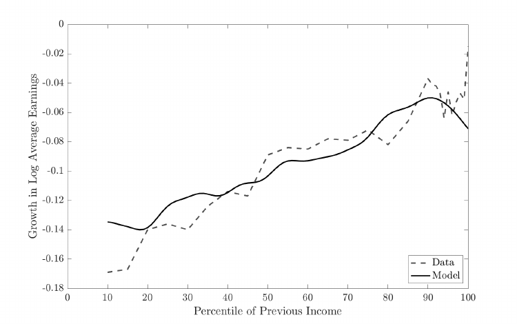
Figure B.1: Incidence of earnings losses during the 1979-1983 recession. The horizontal axis ranks

individuals according to their earnings during 1974-1978. For each percentile of this distribution,

the vertical axis shows the change from 1979 to 1983 in the log of average earnings for that group.

The upward slope implies that lower-income individuals suﬀered larger earnings losses on average in

the recession. Data are taken from Guvenen et al. (2014). The model results are from a simulation

of the ﬁtted income process, feeding in the time series of average (aggregate) earnings growth.

monetary policy shocks: the relative risk aversion γ and the Phillips curve slope κ. We use

the high-frequency monetary shocks identiﬁed by Gertler & Karadi (2015) to estimate the

response of key macro aggregates to identiﬁed monetary shocks. We ﬁrst describe the results

and internal calibration procedure and then give the details of the empirical implementation.

Figure B.2 shows point estimates for four estimated impulse response functions. In the

left panel we show the time path of real interest rates, which we construct as i

− π

t+1

As expected, the expansionary monetary shock leads to a persistent decline in real interest

rates. The center panel shows that consumption increases, eventually reaching a peak of

0.9% above steady state. The right panel reveals that inﬂation rises quite persistently, with

a peak increase of about 0.3%.

Our internal calibration procedure assumes that monetary policy is set according to a

standard Taylor rule subject to shocks. We ﬁnd a path of current and anticipated monetary

policy shocks that, when announced at date 0, leads to a change in real rate expectations that

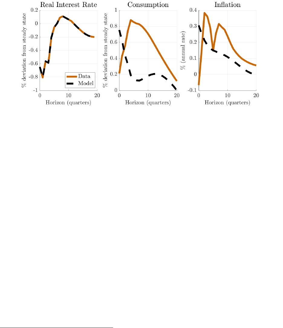
Figure B.2: Empirical (orange) and model-implied (blue-dashed) impulse response following an

expansionary monetary policy shock.

perfectly replicates the empirical estimate in Figure B.2.

We then choose {γ, κ} to match

the peak responses of output and inﬂation. Figure B.2 shows the model-implied impulse

response functions. For output and inﬂation, the model generates the correct peak response,

but unsurprisingly does not generate the hump-shaped pattern of the empirical estimates.

Our empirical analysis uses the following series: the 3-month Treasury rate, the inﬂation

rate constructed from the log diﬀerence in the GDP deﬂator, and log real GDP per capita.

Our monetary shock series is equal to the OLS point estimates of monetary shocks as implied

by the Gertler & Karadi SVAR-IV, estimated only for scheduled FOMC meetings. We use

data from 1980Q3 to 2015Q3, and estimate the impulse response functions using a recursive

VAR with the identiﬁed shock ordered ﬁrst (Plagborg-Møller & Wolf, 2021).

B.2 Initial asset positions and revaluation eﬀects

At date 0, news arrives that changes the returns on capital, long-term bonds, and capital

bonds away from the steady state return. To allocate these revaluation eﬀects across house-

holds we need to know their steady state gross positions in these three asset classes. Our

approach is to impute these as functions of household net worth based on data from the 2019

By the results in McKay & Wolf (2023), the output of this procedure is independent of the baseline

policy rule, as long as it induces a determinate, sunspot-free equilibrium. Our choice of baseline rule is thus

a purely computational device.

In Figure B.2 we plot W ≡ log(P W/P Y ) + log(Y ), where P W is nominal net worth, P Y is nominal

GDP and Y is real GDP.

SCF. Auclert & Rognlie (2018) use a related approach.

To give an overview, for each household in the SCF we do a calculation that is similar

to the one reported in Table 2. We take the “real world” asset classes and map them into

model assets. We then create ﬁne bins of households by net worth and compute average

portfolios at diﬀerent levels of net worth. We then ﬁt piece-wise polynomials through these

functions of net worth and use these to impute the portfolios of the households in the model

according to their net worth.

In our model, all capital holdings are liquid while in reality consumer durables and

real estate is illiquid. We assume that all households with negative net worth simply have

short-term debt and no long-term debt or capital. As these households tend to be liquidity

constrained in our model, this assumption avoids counterfactually strong spending responses

out of changes in asset values for these households. What follows then applies to households

with positive net worth.

Turning to the details, we use the summary extract of the SCF produced by the Federal

Reserve and the variable names here refer to the variable names there. Deﬁne equity =

stocks+stmutf + 0.5 ∗comutf + bus, where we assume combination and other mutual funds

are 50-50 stocks and bonds. Note that equity includes both public and private equity. Deﬁne

mortgage = nh mort + resdbt + heloc. Deﬁne capital = (nfin − bus + 1.32 × equity), where

1.32 is the leverage ratio for equity and nfin − bus is real estate and consumer durables

(non-ﬁnancial assets less business holdings). Deﬁne short term bond holdings as short =

liq+cds−ccbal−install−0.38∗0.32×equity−0.5∗mortgage). This sums cash-like accounts

less credit card and installment loans. We then subtract oﬀ the short-term debt associated

with the leveraged position in capital

and half of the mortgage balance. Finally, we deﬁne

long = bond+tfbmutf +gbmutf +obmutf +0.5∗comutf −0.62∗0.32∗equity−0.5∗mortgage.

We rescale all dollar values so that average household income is 1. We then take averages

within ﬁne bins of net worth. We then perform a piecewise regression of the portfolios on a

quadratic function of net worth. We perform this regression separately for households with

net worth above and below one year’s average income.

Like the Distributional Financial Accounts, we use the Financial Accounts for aggregate

quantities of each asset. Therefore, the total stocks of capital, short-term bonds, and long-

term bonds are the totals from Table 2. Our imputation procedure will not exactly match

these totals both because the SCF does not aggregate to the same totals as the Financial Ac-

Every dollar of equity is 1.32 dollars of capital and -0.32 dollars of bonds. Those bonds are 62% long-term

and 38% short term.

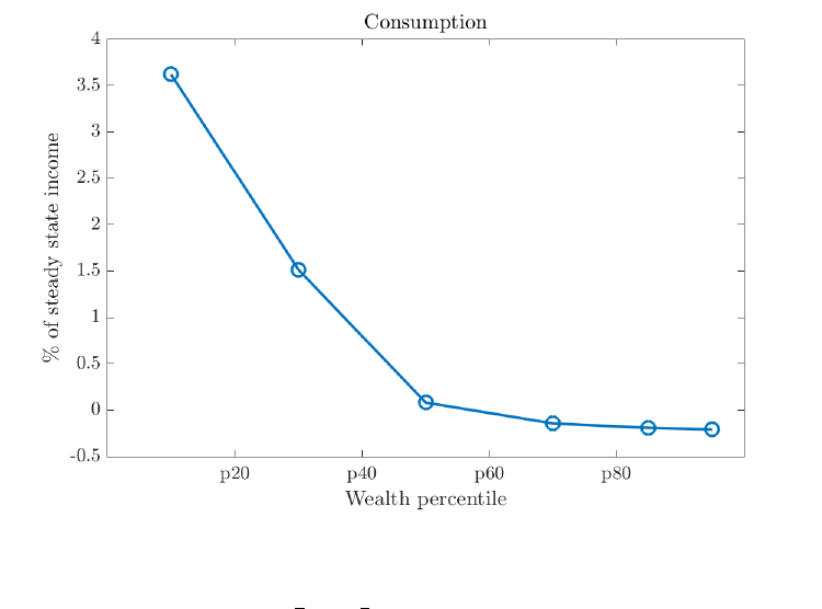
Figure B.3: Initial response of consumption to a $500 ﬁscal stimulus payment across the income

distribution. The ﬁgure includes general equilibrium eﬀects where monetary policy is assumed to

follow a simple interest rate rule i

counts and because our model-generated distribution of net worth does not perfectly match

the SCF distribution of net worth. We therefore rescale the bond positions to match the

total stocks of these assets. We then set capital as net worth less bond holdings. The result-

ing distribution of capital holdings aggregates to the correct total because in the stationary

equilibrium of the economy the total holdings of assets matches the total from Table 2 and if

we have the correct total bond holdings we residually have the correct total capital holdings.

B.3 Additional optimal policy results

We here collect some ﬁgures that supplement the quantitative optimal policy analysis pre-

sented in Section 5.4.

Distributional effects of stimulus checks. Stimulus checks and interest rate cuts

have the same eﬀects on aggregate output and inﬂation (Wolf, 2021), but they diﬀer substan-

tially in their cross-sectional incidence. Figure 2 in the main text shows the model-implied

incidence proﬁle of interest rate cuts; Figure B.3 here does the same for stimulus checks. As

expected, the incidence proﬁle here is strongly downward-sloping: the consumption of poor

households responds the most, reﬂecting their high MPCs and low overall income.

Figure B.4: Simulation of income distribution shock using ad hoc policy rule that stabilizes the

consumption of households with low wealth and low income. The bottom panel shows the con-

sumption of wealthy households increases substantially under this rule leading output and inﬂation

to exceed their targets.

Stabilizing consumption at the bottom. What happens if monetary policy is used

to stabilize consumption of poor households in the face of our distributional shock m

? In

Figure B.4 we plot the implications of following a monetary policy targeting rule that adds

a distributional consideration to the dual mandate targeting rule that seeks to stabilize

the consumption of households with low wealth and low income.

As the ﬁgure shows,

output and inﬂation exceed the dual-mandate targets and the consumption of high-wealth

households is substantially above the steady state level.

The targeting rule is ˆπ

¯η

(ˆy

− ˆy

t−1

) +

ˆc

Low

= 0, where c

Low

is the aggregated consumption of

households with income in the bottom third of the income distribution and wealth below the median.

B.4 Comparison with Bhandari et al. (2021)

In this section we explore further the reasons for why our conclusions on optimal Ramsey

monetary policy following a cost-push shock diﬀer from those of Bhandari et al. (2021).

We argue that the diﬀerences in policy conclusions are due to diﬀerences in the economic

environment. To do so we proceed in two steps. First, we present a model closer to that of

Bhandari et al.. Second, we repeat our optimal policy analysis in that environment.

Environment. We alter our baseline model to arrive at the following alternative environ-

ment, designed to mimic key properties of the model of Bhandari et al.. The changes to the

environment are as follows:

• Proﬁts. We now assume that proﬁts are distributed to households as a function of

their histories of idiosyncratic shocks. In particular, a household receives a share of

their proﬁts equal to the steady state wealth share of a household with that history of

shocks. These claims on future proﬁts are not traded.

• Other assets. The alternative model omits capital in production and includes only

short-term nominal bonds, so there are no traded long-term assets. As we omit capital,

we reduce the total supply of assets, which we now set equal to the steady-state supply

of bonds in Bhandari et al..

• Income process. With fewer assets, our income process—which was calibrated to match

the wealth distribution in our full model—now produces far too many borrowing con-

strained agents. Therefore we use a simpler income process without super-star earners.

• Business-cycle incidence. The alternative model omits the unequal incidence of the

aggregate business cycle across levels of labor income, again in keeping with the baseline

model in Bhandari et al..

Results. We begin by showing that, in this alternative model, monetary policy has strong

distributional eﬀects. Mirroring Figure 2 from our main analysis, Figure B.5 displays the ini-

tial consumption response to an expansionary monetary policy shock across levels of wealth.

We see that, in the alternative environment, there is a clear diﬀerence in shock incidence

across wealth levels, with low-wealth households increasing consumption strongly and high-

wealth households leaving consumption unchanged. This pattern stands in sharp contrast

to Figure 2, where consumption increases evenly across wealth levels.

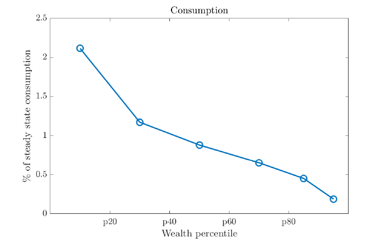
Figure B.5: Initial response of consumption to an expansionary monetary policy shock across the

distribution of wealth in the alternative model described in Appendix B.4.

Next, Figure B.6 shows the optimal policy response to an inﬂationary cost-push shock

in the alternative model. Crucially, and mirroring the ﬁndings of Bhandari et al., we see

that here short-term interest rates fall on impact following the inﬂationary shock. Overall,

the policy response is thus notably more accommodative than the dual mandate policy,

with a shallower fall in output and —given our ﬂat Phillips curve—a modest increase in

inﬂation. In the lower panel we see why the Ramsey policymaker ﬁnds such an aggressive

rate cut optimal: the cost push shock has a distinct distributional gradient, with high-wealth

households increasing consumption and low-wealth households decreasing consumption, and

a rate cut can mitigate this distributional gradient relative to the dual-mandate outcome.

Figure B.6: Optimal policy response to an inﬂationary cost-push shock in the alternative model

described in Appendix B.4.

C Computational appendix

This appendix provides supplementary information on our computational approach. We

compute sequence-space transition paths using the methodology developed in Auclert et al.

(2021), as discussed further in Appendix C.1. Our computation of the inequality term in

the full Ramsey loss function is described in Appendix C.2.

C.1 General equilibrium transition paths

The baseline constraints (2) in our linear-quadratic policy problem in Section 2 are expressed

in sequence space. To compute the corresponding constraints (21) - (22) for our “HANK”

model, we thus follow the computational techniques of Auclert et al. (2021) to compute the

required sequence-space Jacobian matrices. In particular, our computation of the C

•

maps

in the augmented HANK “IS curve” (22) leverages the so-called “fake news” algorithm.

For computation of the alternative (but equivalent) constraint formulations (25) - (36)

in impulse response space, we follow McKay & Wolf (2023) and proceed as follows. First,

we close the model with arbitrary policy rules for the two instruments i

i and τ

, subject

only to the requirement that the two rules induce a unique equilibrium. We then compute

impulse responses of all policy targets to the full menu of contemporaneous and news shocks

to those two policy rules. Now denote the impulse response matrix of some variable x

shocks to the rule for instrument z

, and similarly write

,ε

for responses to

non-policy shocks ε

under the (arbitrary) baseline rule. Finally write

for the impulse

response matrix of the instrument itself. We then deﬁne Θ

≡

−1

and similarly

,ε

≡

,ε

−1

. The results in McKay & Wolf (2023) imply that the resulting impulse

responses are independent of the chosen baseline policy rule.

C.2 Inequality term

The inequality term says that the planner would like to stabilize a very large number of

targets—one for each history ζ. Both for intuition and for computation, it is useful to observe

that these consumption shares will only ﬂuctuate if the inputs to the household’s decision

problem ﬂuctuate. By our discussion of the consumption-savings problem in Section 3.1,

those inputs include total labor income (equal to y

y), the return on savings (r

r), transfers

(τ

and τ

), the inequality shock (m

m), the initial inﬂation rate π

, and the initial asset

prices q

and q

. In this section we leverage this insight to recast the problem of stabilizing

consumption shares as one of stabilizing the inputs to the household consumption-savings

decision, thus giving the representation in (37), couched in terms of a small number of

aggregates rather than a distribution of histories.

Reformulating the inequality term. Let x

x = (y

y, r

r,τ

,τ

m, π

, q

) be the stacked

sequences of inputs to the household problem. Our goal is to show that there is symmetric

matrix Q such that

∞

t=0

bω

(ζ, x

¯ω(ζ)

dΓ(ζ) =

x + O(||

x||

where here we have been explicit that the consumption shares at date t depend on the full

sequences of inputs x

x. To arrive at this representation, consider a ﬁrst-order approximation

to the time-t consumption share of individuals with history ζ:

bω

(ζ, x

x) ≈ Ω

(ζ)

where the derivative Ω

(ζ) will be deﬁned formally below. This yields

bω

(ζ

¯ω(ζ

)

Ω

(ζ

)

Ω

(ζ

)

¯ω(ζ

)

| {z }

≡Q

(ζ

)

x + O(||

x||

We then integrate across histories and take the discounted sum across time to arrive at

∞

t=0

bω

(ζ

¯ω(ζ

)

dΓ(ζ

) =

∞

t=0

(ζ

)dΓ(ζ

)

| {z }

≡Q

x + O(||

x||

giving the desired representation. We have thus arrived at a representation that almost ﬁts

into our general linear-quadratic set-up of Section 2.1, the sole diﬀerence being that the

objective function features a non-diagonal quadratic form. To extend our optimal policy

results to this more general case, we consider the same problem as in Section 2.1, but

replacing the diagonal loss function (1) by the more general (non-diagonal) expression

L ≡

x, (C.1)

The corresponding necessary and suﬃcient ﬁrst-order conditions yield the more general op-

timal policy targeting rule

x = 0

and the optimal instrument path

∗

≡ −



x,z

P Θ

x,z



−1



x,z

P Θ

x,ε

· ε



Evolution of consumption shares. We now explain the ﬁrst-order approximation of

consumption shares

bω

(ζ

) ≈ Ω

(ζ

that we used above. Let c

(ζ

x) be the consumption in date t after history ζ

with the input

sequences given by x

x, and similarly let a

t+1

(ζ

x) be the savings chosen in date t. Also let

be the date-t value of the idiosyncratic state. Using the standard recursive representation

of the household’s problem, we can write these choices in terms policy functions, f and g,

that take as their arguments assets a

(ζ

t−1

) and the current shock ζ

, so we have

(ζ

x) = f



(ζ

t−1

x), ζ



(C.2)

t+1

(ζ

x) = g



(ζ

t−1

x), ζ



. (C.3)

We now consider a ﬁrst-order approximation to f and g around x

x =

(ζ

x) ≈ ¯c(ζ

) +

(ζ

t+1

(ζ

x) ≈ ¯a(ζ

) +

t+1

(ζ

The derivatives that appear here are total derivatives with respect to x

x, including both the

eﬀect on the policy rule at date t and the eﬀect on assets a

(ζ

t−1

x). The derivatives are

evaluated at the steady-state inputs

x and the level of assets that an individual with history

would have if the inputs x remained at steady state forever, which we denote by ¯a(ζ

t−1

To calculate these derivatives, we diﬀerentiate (C.2) and (C.3):

(ζ

∂f

(¯a

(ζ

t−1

), ζ

∂a

(ζ

t−1

∂f

(¯a

(ζ

t−1

), ζ

∂x

(C.4)

t+1

(ζ

∂g

(¯a

(ζ

t−1

), ζ

∂a

(ζ

t−1

∂g

(¯a

(ζ

t−1

), ζ

∂x

. (C.5)

The partial derivative

∂f

¯a

(ζ

t−1

),ζ

)

∂a

is the marginal propensity to consume for an individual

with states (¯a

(ζ

t−1

), ζ

) in the stationary equilibrium, and

∂g

¯a

(ζ

t−1

),ζ

)

∂a

is the marginal

propensity to save. Similarly, the partial derivative

∂f

¯a

(ζ

t−1

),ζ

)

∂x

is the derivative of the

consumption policy rule with respect to the input sequences for an individual with the same

states, and

∂g

¯a

(ζ

t−1

),ζ

)

∂x

is the analogous derivative of the savings policy rule.

We discuss below how to compute these derivatives. Given that they have been recovered,

it remains to move from consumption levels to consumption shares:

(ζ

x) ≡

(ζ

x)dΓ

(ζ)

≈ ¯ω

(ζ

) +

¯c

(ζ

x −

¯c(ζ

)

¯c

(ζ

dΓ(ζ

)

Ω

(ζ

) is then given by

Ω

(ζ

) ≡

¯c

(ζ

−

¯c(ζ

)

¯c

(ζ

dΓ(ζ

). (C.6)

Computing Q. To compute Ω

(ζ

) and so Q, the key challenge is to arrive at the deriva-

tives in (C.4) - (C.5). To do so we begin by simulating a history ζ

for t = 0, 1, ..., T in a

stationary equilibrium (i.e. with x

x =

x). At each date along this simulation, we recover

the required partial derivatives as follows. The marginal propensities to consume and save

can be computed by standard methods. For the derivatives of the policy rules, we use the

fact that the derivatives with respect to past prices are zero and the derivatives with respect

to current and future prices only depends on the number of periods until the price change

occurs. This allows us to compute all the derivatives by perturbing prices at a single date

and iterating backwards in time using a single loop from T to 0 (see Auclert et al., 2021).

With the partial derivatives in hand, we then construct

(ζ

and

t+1

(ζ

by iterating

(C.4)-(C.5) forward starting with

(ζ

−1

given by the change in the households assets with

the initial asset prices (the revaluation eﬀects). Given those derivatives, we can recover Ω

(ζ)

and thus get Q

(ζ

) as well as Q itself.

Impulse response representation. Using (C.4), (C.5), and (C.6), we can write ω

(ζ)

as a linear function of the aggregate variables contained in x

x. Since each ω

(ζ) is linearly

related to x

x, and since we can recover the entries of x

x as a function of (y

y, π

π, i

i,τ

m) (by

Lemma 1), we recover the impulse response representation in (35).

D Proofs and auxiliary lemmas

D.1 Proof of Lemma 1

We begin the proof by re-stating and slightly simplifying the deﬁnition of an equilibrium in

Deﬁnition 1. We ﬁrst repeat the Phillips curve in stacked form:

π = Π

y + ψη

η, (D.1)

where







1 −β 0 · · ·

0 1 −β · · ·

0 0 1 · · ·







, Π

= κI.

Turning to the demand side, we re-write (18) and goods market clearing as

y =

¯c

¯y

+ C

)

y + C

r + C

+ C

m + C



π + H

+ H

i

(D.2)

where e

= (1, 0, 0, . . . )

and we have used that by

= (¯c/¯y)bc

. Next, using (14), (15), and

(16), we write the relationships between asset prices and rates of return as

r = r(

π) (D.3)

= q

(

π,

r) (D.4)

= q

(

r) (D.5)

Finally, we combine the government budget constraint (19) and the law of motion for gov-

ernment debt (20) and solve for τ

e,t

to obtain

= τ

(

π,

r). (D.6)

Our ﬁrst auxiliary result is that, given the shocks (m

m,η

η) and policy choices (i

i,τ

), a list

y, r

r,τ

,π

π, q

q) is part of an equilibrium if and only if (D.1) - (D.6) hold. To show this we need

to check the conditions of Deﬁnition 1: requirement 1 and goods market clearing hold by the

construction of (D.2); requirement 3 is re-stated in (D.1); requirement 6 is imposed by (D.6);

requirement 5 is imposed by (D.3)-(D.5); and asset market clearing holds by Walras’ Law.

Finally, to complete the equilibrium let bw and

` be determined by (10) and the linearized

version of (13) so requirements 2 and 4 hold by construction.

We now simplify this characterization of equilibria further to arrive at Lemma 1. The

key step in the argument is to solve out the asset-pricing and government ﬁnancing rules and

plug them into (D.2). First, given

π and

i, we can recover

r from (D.3). We can recover

from (D.4) and

from (D.5). Second, given

π and

, we can recover

from (D.6).

We can thus write

y =

¯c

¯y

+ C

)

y + C

π) + C

+ C

(

π,

m + C



π + H

(

π,

i) + H

(

π)

i

and so

y =

¯c

¯y



+ C



+ H



+ C



| {z }

y +

¯c

¯y



+ C



+ H



| {z }

(D.7)

¯c

¯y



+ C



+ H



| {z }

i +

¯c

¯y

+ C

]

| {z }

¯c

¯y

where T

•

, R

•

, Q

•

, and Q

•

are derivative matrices for

r(•),

(•),

(•), and

(•). (D.7)

embeds (14), (15), (16), and (D.6). We have thus reduced the equilibrium characterization

from statements about (y

y, r

r,τ

,π

π, q

) to statements about (y

y, π

π), establishing the claim.

D.2 Proof of Proposition 1

In light of Lemma 1, we can re-state the optimal policy problem as minimizing (24) subject

to the two constraints (D.1) and (D.7). This problem gives the following necessary and

suﬃcient ﬁrst-order conditions:

π + Π

Wϕ

−

Wϕ

= 0

0 (D.8)

y − Π

Wϕ

+ (I −

)Wϕ

= 0

0 (D.9)

−

Wϕ

= 0

0, (D.10)

where ϕ

and ϕ

are sequences of Lagrange multipliers on the two constraints. The proof of

Proposition 1 proceeds by guessing (and then verifying) that ϕ

= 0

0. Under this assumption,

we can combine (D.8) - (D.9) to get

π + λ

−1

(Π

)

−1

y = 0

It is straightforward to verify that this can be re-written as

π +







1 0 0 . . .

−1 1 0 . . .

0 −1 1 . . .







y = 0

0 (D.11)

But this is just (28), with the conclusion following for t = 0 since by

−1

= 0 (as the economy

starts from steady state). It now remains to verify the guess that ϕ

= 0

0. For this, consider

some arbitrary (m

m,η

η), and let (

∗

) denote the solution of the system (D.1) and (D.11)

given (m

m,η

η). It remains to show that condition (27) is precisely suﬃcient to ensure that we

can always ﬁnd

i such that (D.7) holds.

Plugging into (D.7) and re-arranging:

∗

−

∗

−

∗

− C

| {z }

demand target

i. (D.12)

Note that the left-hand side of (D.12) is an excess demand term: supply

∗

vs. demand

∗

+ C

m. At this point, as long as

is invertible we could stop and say that

whatever the demand target, there is a

i that satisﬁes (D.12). Invertibility of

is too

restrictive, however, as we can say that the demand target will satisfy certain conditions so

i does not need to be able to generate any possible sequence.

By construction of the

C function,

, and

map into zero-NPV sequences and

preserves the NPV of

y. So equation (D.12) has a particular structure: both sides are

zero-NPV sequences. Provided that all zero-NPV sequences are in the image of

there

exists a

i that satisﬁes (D.12).

D.3 Proof of Proposition 2

Let U

denote the time-t ﬂow utility of the Ramsey planner. To derive the second-order

approximation to the social welfare function, it is convenient to begin by writing U

in terms

of log deviations of c

and `

from steady state:

ϕ(ζ)



¯ce

(ζ)



1−γ

− 1

1 − γ

dΓ(ζ) − ν





. (D.13)

Our objective is to construct a second-order approximation of (D.13). Similar to the analysis

in Woodford (2003), our strategy is to consider an eﬃcient steady state, allowing evalua-

tion of Equation (D.13) to second order using only a ﬁrst-order approximation of aggregate

equilibrium dynamics.

Optimality of the steady state requires that the weighted marginal utility of consumption

is equalized across histories:

ϕ(ζ)¯c

1−γ

¯ω(ζ)

−γ

= ¯u

¯c ∀ζ

for some constant ¯u

. Rearranging, we can write this as

ϕ(ζ)

1/γ

= ¯c¯ω(ζ)¯u

1/γ

∀ζ

Furthermore imposing that consumption shares integrate to 1 yields

ϕ(ζ)

1/γ

dΓ(ζ) = ¯c¯u

1/γ

. (D.14)

Combining the previous two equations, we can recover consumption shares as a function of

planner weights:

¯ω(ζ) =

ϕ(ζ)

1/γ

ϕ(ζ)

1/γ

dΓ(ζ)

∀ζ

For future reference it will furthermore be useful to deﬁne

Ξ ≡



ϕ(ζ)

1/γ

dΓ(ζ)



= ϕ(ζ)¯ω(ζ)

−γ

∀ζ. (D.15)

With these preliminary deﬁnitions out of the way, we can begin constructing the second-

order approximation of (D.13). Diﬀerentiating U

with respect to bc

, we ﬁnd that

∂U

∂bc

ϕ(ζ)(¯c¯ω(ζ))

1−γ

dΓ(ζ)

= ¯c

1−γ

where the second line follows from the deﬁnition of Ξ and some algebra. Notice that the

deﬁnition of Ξ and (D.14) together imply that Ξ = ¯u

/¯c

−γ

so Ξ is the ratio of the (common)

marginal utility of consumption as evaluated by the planner and the marginal utility of

aggregate consumption used by the labor union to value income gains. Next we have

∂U

∂

= −ν

(

The total level of production in steady state is eﬃcient by virtue of the assumed pro-

duction subsidy. To see this, ﬁrst note that the planner’s problem is to choose c and ` to

maximizing welfare subject to ¯c = Ak

1−α

− δk. This leads to the eﬃciency condition

¯c

−γ

Ξ (1 − α) Ak

−α

= ν

(

`).

For future reference, it is useful to re-express this as

¯c

1−γ

Ξ = (1 − α)

−1

¯c

¯y

(

`. (D.16)

Turning to the decentralized equilibrium, it follows from the steady state versions of equations

(13), (10), and (A.3)-(A.5) that Ξ¯c

−γ

= ν

. That the same eﬃciency condition holds.

Diﬀerentiating U

with respect to the consumption shares ω

(ζ) we have

∂U

∂ω

(ζ)

= ϕ(ζ)¯c

1−γ

¯ω(ζ)

−γ

dΓ(ζ)

= ¯c

1−γ

ΞdΓ(ζ)

Turning to second order terms, we begin again with the total level and cross-sectional

split of consumption. We ﬁnd

∂

∂bc

= (1 − γ)Ξ¯c

1−γ

∂

∂ω

(ζ)

= −γ¯c

1−γ

¯ω(ζ)

dΓ(ζ)

∂

∂bc

∂ω

(ζ)

= (1 − γ)Ξ¯c

1−γ

dΓ(ζ)

For hours worked we have

∂

= −ν

(

− ν

(

We can now put everything together, giving the following second-order approximation of

time-t planner utility (D.13):

≈

U + ¯c

1−γ

Ξbc

− ν

(

(1 − γ)Ξ¯c

1−γ

−



(

+ ν

(



−

γ¯c

1−γ

bω(ζ)

¯ω(ζ)

dΓ(ζ)

+¯c

1−γ

bω

(ζ)dΓ(ζ) + (1 − γ)¯c

1−γ

Ξbc

bω

(ζ)dΓ(ζ)

Since consumption shares integrate to 1, it follows that

bω

(ζ)dΓ(ζ) = 0, and so all terms

in the last row are zero. We now wish to evaluate the remaining terms to second order. To

begin, note that the resource constraint and production function give

¯y

¯c

¯y

¯c

(1 − α)

−

(1 − α)

−1



¯c

¯y



Substituting this in for

everywhere we have

≈

U + ¯c

1−γ

Ξbc

− ν

(

`(1 − α)

−1



¯c

¯y



(1 − γ)Ξ¯c

1−γ

−

(φ + 1) ν

(

`(1 − α)

−2



¯c

¯y



−

γ¯c

1−γ

bω(ζ)

¯ω(ζ)

dΓ(ζ)

where we have used the deﬁnition of φ. To simplify this expression further, impose the

aggregate resource constraint bc

¯y

¯c

, use (D.16), and ﬁnally note that all higher-order

price dispersion terms can be ignored to second order. We thus get

≈

U + ν

(

`(1 − α)

−1



−

(1 − α)

−1

(1 − γ)(1 − α)

¯y

¯c

− (φ + 1)

−

¯c

¯y

bω(ζ)

¯ω(ζ)

dΓ(ζ)



The last step in the derivation is to express

in terms of the history of inﬂation, closely

following the arguments in Woodford (2003). The dispersion term is deﬁned as

≡





−η





−η

dj,

where we have deﬁned bp

as the log of p

. Taking a second-order approximation around

= ¯p

≡ E

[log p

] and η

= ¯η yields

≈

−¯η(bp

− ¯p

) +



¯η

(bp

− ¯p

)

− 2(bp

− ¯p

)bη



¯η

Var

[bp

]

where we have simpliﬁed using that fact that, at our expansion point, there is no dispersion

in p

, so e

= ¯p

∀j. Next we use the Calvo structure to rewrite the deﬁnition of d

= θ



jt−1

t−1



−η

dj (1 + π

)

+ (1 − θ)



1 − θ

−

1 − θ

(1 + π

)

−1



/(η

−1)

A second-order approximation of this expression (around a zero-inﬂation steady state) yields

≈ θ

¯η

Var

[bp

jt−1

] +

θ¯η

2(1 − θ)

bπ

≈ θ

t−1

θ¯η

2(1 − θ)

bπ

Solving backwards:

≈ θ

t+1

−1

θ¯η

2(1 − θ)

s=0

t−s

bπ

(D.17)

The aggregate production function is obtained from integrating (A.1) across j and using (13), the fact

that all ﬁrms choose the same capital-labor ratio, and labor market clearing.

We can now return to the problem of the planner. Using our results so far, we can write

planner preferences as

∞

t=0

≈ −

(

1 − α

∞

t=0



(γ − 1)

¯y

¯c

φ + 1

1 − α



¯c

¯y

bω(ζ

)

¯ω(ζ

)

dΓ(ζ

)



Note that bπ

aﬀects

, β

t+1

, · · · by

θ¯η

2(1−θ)

(1, βθ, · · · ) so the discounted sum is

θ¯η

2(1−θ)(1−βθ)

Using this we have

∞

t=0

≈ −

(

1 − α

∞

t=0



θ¯η

2(1 − θ)(1 − βθ)

bπ



(γ − 1)

¯y

¯c

φ + 1

1 − α



¯c

¯y

bω(ζ

)

¯ω(ζ

)

dΓ(ζ

)



= −

(

`θ¯η

2(1 − α)(1 − θ)(1 − βθ)

∞

t=0



bπ

˜κ

¯η

(1 − θ)(1 − βθ)γ

¯ηθ

¯c

¯y

bω(ζ

)

¯ω(ζ

)

dΓ(ζ

)



(D.18)

where

˜κ ≡



(γ − 1)

¯y

¯c

φ + 1

1 − α



(1 − θ)(1 − βθ)

D.4 Auxiliary lemma for Proposition A.1

We here establish that, under Assumptions A.1 to A.3, changes in nominal interest rates

do not aﬀect the distribution of consumption shares. We proceed in two steps. First, we

show that consumption dispersion is unaﬀected by changes in real interest rates and output

that satisfy particular conditions. Second, we establish that changes in the monetary policy

stance induce changes in real interest rates and output that satisfy precisely those conditions.

Throughout, our arguments closely follow Werning (2015).

Lemma D.1. Suppose that Assumptions A.1 to A.3 hold, and consider paths (r

r,y

y, m

m,τ

)

such that

m = τ

= 0

0 and, for all t = 0, 1, 2, . . . ,

−1

β(1 + r

t+1

−1

t+1

, (D.19)

where

β ≡ (1 + ¯r)

−1

. Then the distribution of consumption shares remains constant at its

steady state distribution: ω

(ζ) = ¯ω(ζ) for all t and ζ.

Proof. We will rewrite the household budget constraint using several substitutions. First,

there are no transfers and no government debt to service so the government budget implies

= 0. Second, we use the acyclical earnings risk from Assumption A.1. Third, as capital

is the only asset traded, the value of assets at the start of period t is a

i,t



αy

/k + q



i,t

where k

i,t

is the units of capital purchased by the household at date t − 1. Similarly, the

value of assets at the end of period t is a

i,t+1

/(1 + r) = q

i,t+1

. Putting the pieces together,

the household budget constraint (8) becomes

i,t+1

+ c



αy

/k + q



i,t

Φ(ζ

, ¯m)(1 − α)y

. (D.20)

Combining the asset-pricing relationship (16) and the aggregate Euler equation (D.19),

we have



t+1



Provided that steady state real rates are positive, we have that

β < 1 and so we can solve

forward to ﬁnd q

βα/

k(1 −

β)

. In steady state, the return on capital implies

¯r¯q

= α¯y/k so we have (using

β = 1/(1 + ¯r))

¯q

¯y

The household budget constraint becomes

¯y

¯q

i,t+1

+ c

= (1 + ¯r) ¯q

¯y

i,t

Φ(ζ

, ¯m)(1 − α)¯y

¯y

. (D.21)

Letting z denote an arbitrary realization of ζ

, we will now re-state the household

consumption-savings problem in recursive form. We have

(k, z) = max

≥0

log

(1 + ¯r)k¯q

Φ(z, ¯m)(1 − α)¯y − ¯q

+ log



¯y



+ βE [V

t+1

, z

)]

If V

t+1

is of the form V

t+1

(k, z) =

V (k, z) + B

t+1

for some sequence B

t+1

, then the Bellman

equation above can be written as

(k, z) = max

≥0

log

(1 + ¯r)k¯q

Φ(z, ¯m)(1 − α)¯y − ¯q

+ βE

V (k

, z

)

+ B

, (D.22)

where B

= log(y

/¯y) + βB

t+1

. As there is no time-varying aggregate variable apart from

, V

satisﬁes the same functional form as V

t+1

. By induction, all previous value functions

satisfy this form. Using the steady-state value function to start the induction (i.e., we start

at the steady-state value function

V (k, z) and B

= 0), we can conclude from (D.22) that

the optimal decision rule for k

as a function of (k, z) will be constant and equal to the

steady state decision rule. This constant decision rule and a stable process for the evolution

of z

implies the distribution of (k

, z

) is stationary. It follows from (D.21) that the optimal

consumption decision rule will scale with y

= c

. This scaling implies consumption shares

are constant and equal to their steady state values.

As a ﬁnal step, it remains to relate this recursive formulation of the household decision

problem to the histories of idiosyncratic events. To this end, note that we can write the

consumption share as a function of the state variables associated with that history:

(ζ) =

c(k(ζ), z(ζ))

¯c

, (D.23)

where c(k, z) is the steady state consumption function, k(ζ) is the steady state capital

holdings of a household with history ζ and z(ζ) is the most recent event in the history ζ.

(D.23) holds for any paths (r

r,y

y, m

m,τ

) such that (D.19) holds and

m = τ

= 0

D.5 Proof of Proposition A.1

It remains to show that changes in nominal interest rates induce paths of r

r and y

y that

satisfy (D.19) (since by linearity we already have

m = τ

= 0

0). But this follows directly

from Werning (2015), as our model economy with Assumptions A.1 to A.3 satisﬁes the

conditions of his result (i.e., acyclical risk and acyclical liquidity). We furthermore note that

our special case is isomorphic to the incomplete markets model that appears in Section IIIB

of Farhi & Werning (2019).

We refer the reader to Werning (2015) for the formal proof.

The model in Farhi & Werning (2019) speciﬁes a particular AR(1) process for idiosyncratic income risk

for the sake of computing numerical solutions. We leave the process more general. The important aspect is

that risk is not aﬀected by monetary policy (see Werning, 2015).

D.6 Proof of Corollary A.1

By (4) we can write the optimal monetary policy rule as

π,i

π +

¯η

y,i

y = 0

0 (D.24)

where we have used the fact that with δ = 0 we have ˜κ = κ. It follows from (D.1) that

π,i

= Π

y,i

(D.25)

and so we can re-write (D.24) as

π +

¯η







1 0 0 . . .

−1 1 0 . . .

0 −1 1 . . .







y = 0

0 (D.26)

giving (A.9).

D.7 Proof of Corollary A.2

We have already shown that the optimal monetary rule is given as (A.9). Since (D.1) also

implies that

π,τ

= Π

y,τ

(D.27)

we can use the same steps as in the proof of Corollary A.1 to rewrite the ﬁrst two terms in

(38) as

π,τ

π +

¯η

y,τ

y =

π +

¯η







1 0 0 . . .

−1 1 0 . . .

0 −1 1 . . .







Imposing (A.9) sets these terms to zero, so Corollary A.2 follows.