Unconventional Monetary Policy According to HANK

Eric Sims

Notre Dame and NBER

Jing Cynthia Wu

Notre Dame and NBER

Ji Zhang

Tsinghua PBCSF

Current draft: August 20, 2022

Abstract

This paper studies the implications of household heterogeneity for the eﬀective-

ness of quantitative easing (QE). We consider a heterogeneous agent New Keynesian

(HANK) model with uninsurable household income risk. Financial intermediaries are

subject to an endogenous leverage constraint that allows QE to matter. We ﬁnd that

macro aggregates react very similarly to a QE shock in the HANK model compared

to a representative agent (RANK) version of the model. This ﬁnding is robust across

diﬀerent micro- and macro- distributions of wealth.

We are grateful to Drew Creal, Soroush Ghazi, Jasmine Xiao, as well as seminar and conference

participants at NBER Summer Institute Monetary Economics Meeting, Penn State University, Tsinghua

University, the University of Alabama, 2022 Renmin University of China School of Finance Workshop,

and Marquette University for helpful comments. Sims and Wu acknowledge support from the National

Science Foundation under Grant No. SES-1949107. Ji acknowledges support from the National Natu-

ral Science Foundation of China (No.72003102). Correspondence: [email protected], [email protected],

[email protected].

1 Introduction

In response to the Great Recession, the Federal Reserve (Fed) lowered its short-term pol-

icy rate to zero. With its conventional stabilization tool unavailable, the Fed resorted to

unconventional policy to provide support to the US economy. The most prominent of its

unconventional policy tools was quantitative easing (QE, also referred to as large scale as-

set purchases, or LSAPs). Purchasing longer-term Treasuries and agency mortgage-backed

securities (MBSs), the Fed more than doubled its balance sheet within the span of a few

months in late 2008. By the time it halted active asset purchases in the middle part of the

2010s, the Fed’s balance sheet had quintupled in size relative to its pre-Great Recession level.

The Fed resumed active asset purchases in 2020 in response to the COVID-19 pandemic,

doubling the size of its balance sheet in less than two years.

There is a large and still growing literature on the eﬀectiveness of QE. Most theoretical

work in this literature is based on representative agent New Keynesian (RANK) models –

see, for example, Gertler and Karadi (2013), Sims and Wu (2020, 2021a), and Sims, Wu

and Zhang (forthcoming). At the same time, there has been signiﬁcant interest in the

implications of micro-level heterogeneity for macroeconomic ﬂuctuations in general, and in

particular with respect to the transmission of monetary policy; i.e., the heterogeneous agent

New Keynesian (HANK) literature (e.g. Kaplan, Moll and Violante 2018, McKay et al.

2016, Auclert 2019, Acharya and Dogra 2020, Alves, Kaplan, Moll and Violante 2020, Ravn

and Sterk 2020, and others). To date, however, this literature has mainly considered the

implications of heterogeneity for conventional monetary policy in the form of movements in

short-term interest rates. The goal of our paper is to marry these two literatures to investigate

whether, and to what extent, household heterogeneity matters for the eﬀectiveness of QE.

The one exception of which we are aware is Cui and Sterk (2021). However, the underlying frictions for

QE to matter diﬀer in the two papers. Our paper follows the QE literature and features frictions on ﬁnancial

intermediaries. QE transmits through intermediaries and impacts the real economy via investment. In

contrast, Cui and Sterk (2021) follow more closely the HANK literature, with two types of assets households

can hold. The main mechanism through which QE works in their model is through household marginal

propensities to consume out of two types of assets, not via intermediaries or through ﬁrm investment.

We develop a quantitative general equilibrium model with household heterogeneity and

scope for QE to matter. Households face uninsurable idiosyncratic unemployment ris and

endogenously supply labor. They may save via short-term deposits with ﬁnancial interme-

diaries, subject to a borrowing constraint, and receive dividends from their ownership in

production ﬁrms and ﬁnancial intermediaries. Financial intermediaries engage in maturity

transformation, standing between households who save via short-term deposits, and produc-

tion ﬁrms who ﬂoat long-term debt to ﬁnance investment. Financial intermediaries face an

endogenous leverage constraint, and production ﬁrms are required to ﬁnance a fraction of

their investment by issuing long-term bonds. Prices and nominal wages are sticky. Central

bank purchases of long-term assets can ease the leverage constraint facing intermediaries,

resulting in lower interest rate spreads and more investment. We refer to an exogenous

increase in central bank long-term asset holdings as a QE shock.

In our benchmark speciﬁcation, we assume that all households receive the same dividend

payout each period. The responses of aggregate variables to a QE shock are nearly identical to

a representative agent (RANK) version of the model, even though the HANK version features

substantial wealth inequality due to uninsurable employment risk and a borrowing constraint.

The only noticeable diﬀerence is the consumption response of the very poorest households

in the HANK version, which increases sharply after a QE shock. But this distributional

diﬀerence has little impact on aggregate variables.

We consider robustness of our results with respect to both the micro- and macro- distri-

butions of wealth. First, regarding the micro distribution, we allow a more general dividend

distribution rule, in which dividends vary, potentially non-linearly, with household wealth.

We explore the implications of this distribution rule for popular inequality metrics, such

as the Lorenz Curve and the Gini Coeﬃcient. With a signiﬁcant gap between dividends

received by the richest and poorest households, and suﬃcient non-linearity in the relation-

ship between dividend receipt and wealth, our model can generate more wealth inequality

compared to our benchmark speciﬁcation. However, diﬀerent degrees of micro-level wealth

inequality matter little for aggregate dynamics. Regardless of how we specify the dividend

distribution rule, we ﬁnd that the impulse responses of aggregate variables to a QE shock

are remarkably similar, and in turn almost identical to a RANK version of the model.

Next, we investigate the extent to which macro parameterizations related to the wealth

distribution inﬂuence the aggregate transmission of QE shocks. When we parameterize

the model so that a higher fraction of the population is unemployed in each period, many

more households are located at or near the borrowing constraint compared to our baseline

speciﬁcation. This results in the aggregate eﬀects of a QE shock being slightly bigger.

These diﬀerences are nevertheless not economically large, and are only visibly noticeable for

very high unemployment rates. We then investigate whether the duration of unemployment

spells matters for the aggregate transmission of QE shocks and ﬁnd it is almost completely

irrelevant. We also examine the role of the unemployment beneﬁt paid out to unemployed

households. Smaller or larger values of this parameter have modest implications for the

stationary wealth distribution, but matter little for the aggregate eﬀects of QE. Finally, we

study the sensitivity of our results to households’ risk aversion. This parameter has little

eﬀect on how QE impacts the economy.

There are two potentially important takeaways from our quantitative exercises. The

ﬁrst is that there seems to be little gained by formally modeling household heterogeneity

if one is interested in is the aggregate eﬀects of a QE shock. Our ﬁnding that RANK is a

good approximation to a substantially more complicated and numerically more demanding

HANK model is consistent with a recent paper by Debortoli and Gali (2022), who argue

that idiosyncratic income uncertainty is unimportant for aggregate ﬂuctuations. Another

important takeaway from our analysis is that there seems to be little connection between

various inequality metrics and aggregate dynamics in response to a QE shock. Much of

the existing literature uses moments such as the Gini coeﬃcient as summary statistics for

inequality. To the extent to which one is only interested in aggregate dynamics, our results

suggest that this focus on inequality metrics might be misplaced.

In addition to these substantive issues, our paper also makes a methodological con-

tribution. Though our model features idiosyncratic income risk, wealth inequality, and a

borrowing constraint, we are able to solve the model using perturbation methods in Dynare,

a popular program for solving, simulating, and estimating RANK models. Our paper is sim-

ilar in this respect to Winberry (2018), who also solves a heterogeneous agent model with

perturbation methods in Dynare. Substantively, our model features nominal rigidities and

other frictions common in the New Keynesian literature, whereas his model ﬁts into a real

business cycle framework. Methodologically, we depart from him in that we follow Young

(2010) to approximate the cross-sectional distribution with a non-parametric histogram,

whereas Winberry (2018) follows Algan et al. (2008) to approximate this distribution within

a parameteric family. The advantage of our approach is that it does not involve numerical

optimization, which slows the calculation when done repeatedly and does not guarantee con-

vergence. Our method is not limited to the QE application on which we focus in this paper,

nor is it speciﬁc to the exact form of household heterogeneity.

The remainder of the paper is organized as follows. Section 2 lays out our model. Section 3

discusses our method for solving the model. Section 4 compares and contrasts impulse

responses to an exogenous QE shock with and without household heterogeneity. Section 5

discuss our model’s implications for popular inequality metrics and considers a more general

form of the dividend distribution rule to study how that aﬀects the aggregate dynamics in

response to a QE shock. Section 6 considers changing macro parameters and investigates

the extent to which they matter for aggregate dynamics in response to a QE shock. The

ﬁnal section concludes.

2 Model

Our model features ﬁnancial frictions, a banking sector, and has scope for central bank

asset purchases to matter. In addition, households are heterogeneous and face uninsurable

unemployment risk. In this section,we provide detail on key elements of the model and

relegate remaining details to Appendix A.

2.1 Households

The household sector is similar to Krusell and Smith (1998), except that labor supply is

endogenous. There are a continuum of households indexed by j ∈ [0, 1]. Each maximizes

the present discounted value of lifetime ﬂow utility:

∞

t=0

log c

j,t

− χ

1+η

j,t

1 + η

, (2.1)

where c

j,t

and l

j,t

are an individual household’s consumption and labor supply. β ∈ (0, 1) is

a discount factor, χ > 0 is a scaling parameter, and η is the inverse Frisch elasticity.

Each household faces an exogenous idiosyncratic labor productivity shock, ε

j,t

∈ {0, 1}.

This productivity shock can be interpreted as an employment shock, where ε

j,t

= 0 indicates

unemployed and consequently l

j,t

= 0, while ε

j,t

= 1 means that the household will earn

a positive market wage and will hence choose to work, l

j,t

> 0. ε

j,t

evolves stochastically

according to a two-state Markov process with the transition matrix







p(ε

j,t+1

= 0|ε

= 0) p(ε

j,t+1

= 1|ε

= 0)

p(ε

j,t+1

= 0|ε

= 1) p(ε

j,t+1

= 1|ε

= 1)













p 1 − p

1−U

(1 − p) 1 −

1−U

(1 − p)







. (2.2)

The aggregate unemployment rate is U = p(ε

j,t

= 0) and is ﬁxed. Total labor supply is

j,t

dj.

Household j saves via deposits, d

j,t

, with ﬁnancial intermediaries, which earn the gross

interest rate, R

, from t to t + 1. Deposits are the only asset the household can accumulate.

A household faces the following ﬂow budget constraint:

j,t

t−1

j,t−1

+ mrs

[(1 − τ)l

j,t

+ µ(1 − ε

j,t

)] − c

j,t

− T

+ div

j,t

− X, (2.3)

where Π

is the gross inﬂation rate, mrs

is the real wage, τ is a tax rate on labor income,

µ × mrs

is an unemployment beneﬁt, T

is a lump-sum tax, and X is a real transfer paid

out to new ﬁnancial intermediaries, to be discussed below. div

j,t

is a dividend transfer from

all ﬁrms. This dividend is taken as given by households; we will discuss how it is distributed

across agents in Section 4 and Section 5. d

j,t

, c

j,t

,and l

j,t

are endogenous choice variables.

Each household faces a borrowing constraint and a constraint on its time endowment:

j,t

≥ d (2.4)

j,t

≤

l. (2.5)

The ﬁrst order conditions are

−1

j,t

≥ βR

−1

j,t+1

t+1

(2.6)

j,t

≤

(1 − τ)mrs

χc

j,t

. (2.7)

The equalities hold when the constraints in (2.4) and (2.5) do not bind.

2.2 Labor Market

We introduce wage rigidity into our model via labor unions. Unions are indexed by h ∈

[0, 1]. These unions purchase labor from households at real wage mrs

, repackage it into

d,t

(h), and sell it to a representative labor contractor at nominal wage, W

(h). The labor

contractor combines diﬀerentiated labor into ﬁnal labor available for production, L

d,t

via a

CES technology. Final labor is sold to a representative production ﬁrm at nominal wage,

Unions are subject to a Calvo-style nominal rigidity. Each period, a union can adjust

its wage, W

(h), with probability 1 − ϕ

, where ϕ

∈ [0, 1]. Non-updated wages can be

indexed to lagged aggregate inﬂation via the parameter γ

∈ [0, 1]. This setup gives rise to

a conventional wage Phillips curve. See the Appendix for details.

2.3 Production

There are four diﬀerent types of ﬁrms in our model. A representative capital goods producer

transforms raw investment goods into new physical capital subject to a convex adjustment

cost. A competitive ﬁnal good producer aggregates retail output into ﬁnal output via a

CES technology and sells it at nominal price, P

. A continuum of retail ﬁrms, indexed

by f ∈ [0, 1], repackage wholesale output and sell it to the ﬁnal good producer at P

(h).

Retailers have market power and are subject to a Calvo-style nominal rigidity, updating

their prices with probability 1 − ϕ

each period. Non-updated prices can be indexed to

lagged inﬂation via the parameter γ

∈ [0, 1]. The representative wholesale ﬁrm accumulates

its own capital, purchases new capital from the capital goods producer, and hires labor from

the labor contractor. It produces wholesale output, Y

m,t

, from capital and labor, and sells

this output to retail ﬁrms at P

m,t

. The wholesale ﬁrm can choose the intensity with which

it utilizes physical capital, u

, the cost of which is faster depreciation.

With the exception of the wholesale ﬁrm, the production side of the model is reasonably

standard, and details are relegated to an appendix. The wholesale ﬁrm accumulates its own

physical capital, K

. It purchases new physical capital,

, from the capital goods producer

at nominal price P

. We require that the wholesale ﬁrm ﬁnance a fraction, ψ ∈ [0, 1], of

its purchases of new physical capital by issuing long-term bonds. As in Woodford (2001),

these long-term bonds take the form of perpetuities with decaying coupon payments. Let

κ ∈ [0, 1] denote the decay parameter for coupon payments. A bond in period t is sold for

dollars and obligates the issuer to a coupon payment of one dollar in t + 1, κ dollars

in t + 2, κ

dollars in t + 3, and so on. The total nominal coupon liability due in t from

all past issuances is denoted by F

m,t−1

; new issuance of bonds in t is therefore denoted by

m,t

− κF

m,t−1

, which generates Q

dollars for the issuer. The “loan in advance” constraint

facing the wholesale ﬁrm is:

ψP

≤ Q

m,t

− κF

m,t−1

). (2.8)

Equation (2.8) distorts standard ﬁrst order conditions related to capital investment and bond

issuance. It therefore generates “investment” and “ﬁnancial” wedges. Fluctuations in these

wedges are the mechanism through which QE-type policies transmit to the real economy.

2.4 Financial Intermediaries

Financial intermediaries are structured similarly to Gertler and Karadi (2011, 2013), and

Sims and Wu (2021a,b). Each period there is a ﬁxed mass of intermediaries indexed by i.

Intermediaries ﬁnance themselves with net worth, N

i,t

, and deposits taken from households,

i,t

. Each period, a fraction 1 − σ, with σ ∈ [0, 1], stochastically exit and return their net

worth to their household owner. They are replaced by an equal number of new intermediaries

that begin with real start up funds of X given to them by their household owner.

Intermediaries hold privately issued bonds, F

i,t

; government issued nominal bonds, B

i,t

;

and interest-bearing reserves, RE

i,t

, which are held on account with the central bank. Gov-

ernment bonds are structured similarly to private long-term bonds and are priced at Q

B,t

The balance sheet condition of a typical intermediary is:

i,t

+ Q

B,t

i,t

+ RE

i,t

= D

i,t

+ N

i,t

(2.9)

A ﬁnancial intermediary accumulates net worth until stochastically exiting. Net worth

for surviving intermediaries evolves according to:

i,t



− R

t−1



t−1

i,t−1



− R

t−1



B,t−1

i,t−1



t−1

− R

t−1



i,t−1

t−1

i,t−1

(2.10)

t−1

is the (gross) interest rate on reserves, which is set by the central bank and known at

t−1. R

t−1

is the deposit rate, which is determined in equilibrium. (R

−R

t−1

), (R

−R

t−1

and (R

t−1

−R

t−1

) are, respectively, the excess returns from holding private bonds, government

bonds, and reserves relative to the cost of funding via deposits. The term R

t−1

i,t−1

measures

the cost-savings from ﬁnancing via net worth as opposed to deposits. R

and R

are the

realized holding period returns on private and government bonds and satisfy:

1 + κQ

t−1

(2.11)

1 + κQ

B,t

B,t−1

(2.12)

The objective of an intermediary is to maximize its expected terminal net worth, where

discounting is by the stochastic discount factor for households who are not at the borrowing

constraint

t,t+1

t+1

. (2.13)

Consider the problem of an intermediary continuing after period t. There is a 1 − σ

probability that it will exit after t + 1, a (1 − σ)σ probability that it will exit after t + 2, and

so on. Accordingly, its objective is

i,t

= max (1 − σ)E

∞

j=1

j−1

t,t+j

i,t+j

, (2.14)

where n

i,t

= N

i,t

is real net worth, with P

the price of ﬁnal output.

Note that while consumption levels will diﬀer for unconstrained households, since (2.6) will hold with

equality, they all have the same stochastic discount factor.

A ﬁnancial intermediary faces a costly enforcement constraint as in Gertler and Karadi

(2011, 2013). A ﬁnancial intermediary can choose to abscond with some assets at the end of a

period rather than continuing as an intermediary. If an intermediary does this, depositors can

recover a fraction of the intermediary’s assets, with the intermediary retaining the rest. For

depositors to be willing to lend to intermediaries, it must not be optimal for the intermediary

to divert funds in this way, which we refer to as going into bankruptcy. Accordingly:

i,t

≥ θ(Q

i,t

+ ∆Q

B,t

i,t

) (2.15)

In (2.15), the right hand side of the inequality represents the (real) funds that a ﬁnancial

intermediary can keep should it choose to enter bankruptcy, while the left hand side is the

value of continuing as an intermediary.

Should it choose to divert, an intermediary can keep

a fraction of its private bonds, θ, and a fraction of government bonds, θ∆, where 0 ≤ ∆ ≤ 1.

We assume that the third type of asset held by intermediaries – reserves – is fully recoverable

by depositors in the event of bankruptcy.

All ﬁnancial intermediaries will behave in the same way with identical optimality condi-

tions. These are

t,t+1

Ω

t+1

−1

t+1



t+1

− R



1 + λ

θ (2.16)

t,t+1

Ω

t+1

−1

t+1



t+1

− R



1 + λ

θ∆ (2.17)

t,t+1

Ω

t+1

−1

t+1



− R



= 0, (2.18)

where

Ω

= 1 − σ + σθϕ

(2.19)

1 + λ

[Λ

t,t+1

Ω

t+1

−1

t+1

. (2.20)

i,t

= F

i,t

and b

i,t

= B

i,t

are real private and government bond holdings, respectively.

(2.16) - (2.18) are the key equilibrium conditions. λ

≥ 0 is the multiplier on the costly

enforcement constraint. If this constraint does not bind, then to ﬁrst order expected returns

on all three types of assets must equal the cost of funds (i.e. the deposit rate). If the costly

enforcement constraint binds, then there will be excess returns of long-term private and

public bonds over the deposit rate. Because reserves are fully recoverable in the event of

liquidation, arbitrage requires that the interest rate on deposits equal the interest rate on

reserves. (2.19) is an auxiliary variable introduced to simplify the analysis.

The value of an intermediary satisﬁes

i,t

= θϕ

i,t

. (2.21)

When the constraint in (2.15) binds,

i,t

+ ∆Q

B,t

i,t

, (2.22)

which is an endogenous leverage ratio, whose equilibrium condition is in (2.20). The con-

straint makes the ﬁnancial intermediary less levered than it would ﬁnd optimal. This en-

dogenous leverage constraint is ultimately what can give rise to excess returns.

One can show from (2.20) that:

θϕ

≥ 1 + λ

(2.23)

If (2.15) does not bind, then λ

t+j

= 0 for all j, which implies that θ

= 1.

Intuitively,

this means that net worth is as valuable to a household as to an intermediary. In this case,

returns on all assets would be equal. Hence, whether an intermediary invests in F

i,t

, D

i,t

would be irrelevant. When the costly enforcement constraint binds, then λ

> 0 and

θϕ

is larger than one. In this case, there exist excess returns on holding long-term assets

In this circumstance, Ω

= 1.

(private and government bonds).

2.5 Fiscal authority

A ﬁscal authority ﬁnances its expenditure by levying lump sum taxes and a labor income tax

on households, from receipt of a transfer, T

cb,t

, from the central bank, and by issuing long-

term bonds. Its expenditure includes purchases of output, G

, and unemployment beneﬁts.

For simplicity, we assume that the government has a ﬁxed real stock of long-term bonds

issued,

. The government’s budget constraint is:

+ Π

−1

+ mrs

µU = T

+ T

cb,t

+ Q

B,t

(1 − κΠ

−1

) + τmrs

(2.24)

2.6 Monetary policy

The central bank controls the interest on reserves R

, which evolves according to a Taylor

(1993)-type interest rate rule:

ln R

= (1 − ρ

) ln R

+ ρ

ln R

t−1

(1 − ρ

) [ϕ

(ln Π

− ln Π) + ϕ

(ln Y

− ln Y

t−1

)] + σ

r,t

, (2.25)

where 0 ≤ ρ

< 1, ϕ

> 1, and ϕ

≥ 0. ϵ

r,t

is a policy shock. We do not formally analyze

the implications of the ZLB in our analysis, but it would be straightforward to do so.

In addition to setting the interest rate on reserves, the central bank can buy and sell long-

term bonds (either privately issued bonds or government bonds). It ﬁnances these holdings

via reserves, which are held in the banking system. The central bank’s balance sheet, in

nominal terms, is:

cb,t

+ Q

B,t

cb,t

= RE

(2.26)

The central bank’s remittance to the ﬁscal authority amounts to

cb,t

= (1 + κQ

) Π

−1

cb,t−1

+ (1 + κQ

B,t

) Π

−1

cb,t−1

− R

t−1

−1

t−1

(2.27)

We model a QE shock as an exogenous and persistent change in central bank bond

holdings. In particular, we assume that real central bank holdings of privately issued bonds,

cb,t

, follow a stationary AR(1) process (and similarly for holdings of real government bonds,

cb,t

ln f

cb,t

= (1 − ρ

+ ρ

ln f

cb,t−1

+ σ

f,t

, (2.28)

where 0 ≤ ρ

< 1 and f

denotes steady state real bond holdings.

If ﬁnancial intermediaries are unconstrained (i.e. (2.15) does not bind), then ﬂuctuations

in central bank bond holdings are irrelevant. But if intermediaries are constrained, then

increases in central bank bond holdings ease the endogenous leverage constraint, resulting in

higher long-term bond prices (equivalently, lower long-term yields). This ﬁlters through to

the real economy by relaxing the loan in advance constraint on wholesale producers, leading

to more investment and higher aggregate demand.

3 Solution Method and Calibration

In this section, we outline our solution method and discuss the parameterization of our

model.

3.1 Solution Method

We solve our model using perturbation methods with the popular software Dynare. Com-

pared to a global solution, perturbation methods can accommodate a large number of state

variables and require less computational time. Though it is standard practice to solve a

RANK model using Dynare, it is not straightforward to do so when there is household

heterogeneity.

Solving the aggregate part of the model via Dynare is straightforward. The key step

we take is to map the equilibrium conditions of individuals’ policy functions and the cross-

sectional distribution into Dynare. We approximate the conditional expectation, the right-

hand side of (2.6), using Chebyshev polynomials (see, for example, Judd 1998):

βR



−1

t+1



≡ T(d

t−1

, ε

) ≈ exp

(

n=0

n,t

(ε

(ξ(d

t−1

))

)

(3.1)

where T

are Chebyshev polynomials and θ

n,t

are loadings. T(d

t−1

, ε

) gives the inverse of

consumption in period t if the borrowing constraint does not bind. We then solve for the

policy function for deposits, labor, and consumption as follows:

= max

(

t−1

+ mrs

[(1 − τ )l

+ µ(1 − ε

)] − T(d

t−1

, ε

)

−1

− T

+ div

− X, d

)

(3.2)

= min

(



(1 − τ )mrs

χc



)

(3.3)

t−1

+ mrs

[(1 − τ )l

+ µ(1 − ε

)] − d

− T

+ div

− X (3.4)

Iterating the policy functions one period forward, we can further express c

t+1

as a function

of T(d

, ε

t+1

) and hence θ

n,t+1

. Therefore, (3.1) becomes the dynamic equation for θ

n,t

. For

details, see Appendix B.

Next, we update the cross-sectional distribution from t to t+1. We use the non-parametric

method proposed by Young (2010) by approximating the joint distribution p(d

, ε

t+1

) with

a histogram over the grid {d

}

m=0

and ε

t+1

= {0, 1}. The transition dynamics for the

cross-sectional distribution are given by:

p(d

, ε

t+1

) =

t−1

p(d

t−1

, ε

)p(ε

t+1

|ε

)p(d

t−1

, ε

), (3.5)

For brevity, we drop j subscript hereafter.

where p(ε

t+1

|ε

) is given in (2.2).

We know d

t−1

, ε

) from the policy function. However, even with d

t−1

on a discrete

grid, d

does not necessarily fall on a grid point. We follow Young (2010) and approximate

p(d

t−1

, ε

) with the d

grid: ﬁnd the two neighboring grids d

′

, d

′

that are closest to

, where m

′

= 0, ...., M − 1. Assign weights to them using

p(d

= d

′

t−1

= d

, ε

) = 1 −

− d

′

− d

′

p(d

= d

′

t−1

= d

, ε

) =

− d

′

− d

′

. (3.6)

With the transition probabilities in (3.6) and (2.2), (3.5) characterizes the dynamics equa-

tions for the joint probability p(d

, ε

t+1

). See Appendix C for the full set of equilibrium

conditions that we feed into Dynare.

For the stationary equilibrium without aggregate shocks, we solve a ﬁxed-point problem

over aggregate deposits, d, and labor supply, L (aggregate consumption is then determined

given the resource constraint). We proceed in steps. First, given guesses of d and L, we

can compute stationary equilibrium values of all aggregate variables. Then we solve for the

stationary equilibrium values of the Chebyshev coeﬃcients; this step is also a ﬁxed point

problem. Third, we solve the stationary distribution p(d, ε) by iterating (3.5) forward on

the discretized grid until convergence. Once we have the distribution from this step and

the policy functions from the Chebyshev step, we can compute updated values of aggregate

deposits,

d, and labor,

L. We then iterate over these steps until d ≈

d and L ≈

L. For

details of solving the stationary equilibrium, see Appendix D.

Our solution method is related to Winberry (2018). He also proposes a methodology

to solve a model with heterogeneous agents in Dynare. The main diﬀerence relative to our

approach is that he approximates the cross-sectional distribution following Algan, Allais and

Haan (2008), who use a parametric family. This methodology requires a large number of

numerical optimizations when solving the stationary equilibrium. The optimization routines

do not guarantee convergence and the computational burden is high. The numerical behavior

of their approach becomes problematic when the distribution is far away from a normal

distribution, which is the case for our application.

We, instead, follow Young (2010), who uses a histogram over a ﬁxed grid to construct

the cross-sectional distribution. In his approach, updating the approximate cross-sectional

distribution is analytical and does not require numerical optimization. Therefore, it works

well with highly skewed distributions like the ones in our paper. One downside of Young’s

(2010) approach is to accurately approximate the distribution, it requires a large number

of state variables in Dynare, which makes adding additional idiosyncratic states diﬃcult, if

not infeasible. Our solution method is also related to Reiter (2009) in the sense that he also

approximates the cross-sectional distribution with a histogram and employ a perturbation

method.

3.2 Calibration

Table 1 lists the parameter values that are unique to the HANK setup. We set U = 0.05,

which is the fraction of households with low productivity (ε = 0), and hence can be inter-

preted as the aggregate unemployment rate. Conditional on being unemployed, the prob-

ability of remaining unemployed, p, is 0.5. This means that the expected unemployment

duration is two quarters. The scaling parameter governing the disutility of labor, χ, is cho-

sen so that steady state labor supply in a representative agent version of the model would

be L

RANK

= 0.95.

The unemployment beneﬁt is set to 40 percent the wage, µ = 0.4, which

follows Shimer (2005). The labor income tax rate is 30% following Kaplan et al. (2018).

d = 0 implies agents are not allowed to borrow, and

l = 1.5 implies the time endowment for

work is 150% of l

RANK

= 1. If we interpret l

RANK

= 1 to eight hours a day,

l = 1.5 means

the maximum amount someone can work is 12 hours a day. For other parameters, we follow

the calibration from Sims and Wu (2021a); see details in Table E.1 of Appendix E.

This could be interpreted as 95 percent of the population supplying l

RANK

= 1 unit of labor each, which

Table 1: Calibration of HANK parameters

Parameters Value Target Description

U 0.05 Fraction unemployed

p 0.5 unemployment duration two quarters Probability of staying unemployed

χ L

RANK

= 1 − U Labor disutility scaling parameter

µ 0.4 Unemployment beneﬁt / wage

τ 0.3 Labor income tax rate

d 0 Borrowing constraint

l 1.5 Time endowment

4 HANK vs RANK

In this section, we compare and contrast impulse responses to a QE shock under both a

RANK and a baseline HANK speciﬁcation.

In the baseline HANK model, we assume

dividends are equally distributed across households; we explore the implications of diﬀerent

distribution rules in Section 5.

Even with this equal distribution rule, there remains signiﬁcant household wealth het-

erogeneity that arises from uninsurable employment/productivity risk. Figure 1 plots the

stationary distribution of wealth across households, where wealth is normalized by the av-

erage steady state labor income. We do so for both unemployed households (solid blue line)

and employed households (dashed red line). Few households are located at the borrowing

constraint in the stationary distribution.

Nevertheless, most households are relatively poor,

with the distribution of wealth highly right skewed. There are a decent number of house-

holds who are quite wealthy and far away from the borrowing constraint. The distribution of

unemployed households is slightly towards the left of that for employed households, implying

that the former are, on average, less wealthy than the latter.

Figure 2 plots impulse responses to a persistent, private QE shock. The shock is scaled to

is comparable to the targeted 5 percent unemployment rate in the HANK speciﬁcation.

The representative household of the RANK model is standard; we discuss the problem facing the house-

hold, and the associated ﬁrst order optimality conditions, in Appendix F.

We do not include the borrowing constraint in the plot because its probability density is inﬁnity by

construction.

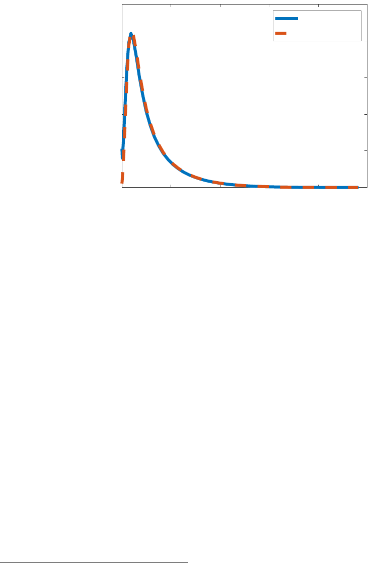
Figure 1: Stationary Distribution

0 20 40 60 80 100

deposit/labor income

0.02

0.04

0.06

0.08

0.1

unemployed

employed

Notes: Blue solid line: unemployed households; red dashed line: employed households. We do not plot the

mass for constrained households. The x-axis measures the ratio between deposits and average steady state

labor income.

represent a four-percent increase in central bank bond holdings.

The solid blue lines show

responses under a RANK version of the model, while the dashed red lines are responses

generated from the HANK speciﬁcation.

The responses of aggregate variables to a shock to central bank bond-holdings in the

RANK speciﬁcation (blue) are similar to Sims and Wu (2021a). Bond purchases ease the

leverage constraint on intermediaries, which results in declining interest rate spreads. This,

in turn, results in more investment. Higher aggregate demand results in output, labor, and

inﬂation all rising temporarily.

For all aggregate variables, the responses under the HANK speciﬁcation (dashed red lines)

are qualitatively and quantitatively similar to the RANK version of the model. Some vari-

ables, including consumption, output, inﬂation, and labor, rise slightly more in the HANK

speciﬁcation on impact, but these diﬀerences are small and short-lived.

This shock generates a similar-sized response of output as to a conventional shock to the policy rule

for the short-term interest rate with a size of 25 basis points; see Figure G.1 in the appendix. As noted in

Appendix E, we assume an autoregressive parameter of 0.8. Responses to a public QE shock (i.e. a purchase

of long-term government bonds, instead of privately-issued bonds), would produce the same-shaped impulse

responses, albeit at a smaller scale.

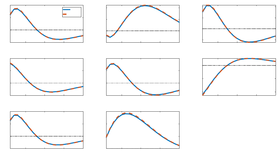
Figure 2: Impulse responses to a QE shock: RANK vs. HANK

5 10 15 20

-0.5

0.5

output

RANK

HANK

5 10 15 20

-0.1

0.1

0.2

consumption

5 10 15 20

-2

investment

5 10 15 20

-0.05

0.05

0.1

inflation

5 10 15 20

-0.05

0.05

0.1

policy rate

5 10 15 20

-0.2

-0.1

corp. bond spread

5 10 15 20

-0.5

0.5

labor

5 10 15 20

0.5

1.5

deposit

Notes: This ﬁgure plots the impulse responses of aggregate variables under a 4% QE shock. The blue solid

lines are for the RANK model, and the red dashed lines are for the HANK model. The x-axis is time in

quarters, and the y-axis is the percentage change from steady state.

We next inspect the reasons for the slight diﬀerences in aggregate responses in the HANK

vs. RANK setups. Figure 3 plots the ﬁrst-period responses of individual choice variables to

a QE shock against the percentile of the wealth distribution. We do so both for a RANK

version of the model (solid blue) and our baseline HANK version (dashed red lines). In the

left panel, we plot the ﬁrst-period responses across the full wealth distribution. To increase

readability, in the right panels we zoom in on responses for households in the bottom one

percent of the wealth distribution. In the RANK model, all households behave identically,

so the ﬁgures simply show ﬂat lines.

For all but the very poorest households, the ﬁrst-period individual responses for con-

sumption, deposits, and labor are almost identical to the RANK counterpart. The poorest

households, in contrast, behave quite diﬀerently. These households increase their consump-

tion and deposits, and reduce their labor supply, following a QE shock. What drives these

results? Households located near the borrowing constraint are working more and consuming

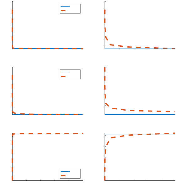
Figure 3: First period individual responses to a QE shock: RANK vs. HANK

0 20 40 60 80 100

0.2

0.4

0.6

0.8

consumption

RANK

HANK

0 20 40 60 80 100

deposit

RANK

HANK

0 20 40 60 80 100

deposit percentile

-0.2

0.2

0.4

0.6

labor

RANK

HANK

0 0.2 0.4 0.6 0.8 1

0.2

0.4

0.6

0.8

consumption

0 0.2 0.4 0.6 0.8 1

deposit

0 0.2 0.4 0.6 0.8 1

deposit percentile

-0.2

0.2

0.4

0.6

labor

Notes: This ﬁgure plots the impulse responses of (employed) individual decision variables (consumption,

deposits, and labor supply) in the period when a 4% positive QE shock hits. The blue solid lines and red

dotted lines are for the RANK and baseline HANK models, respectively. The x-axis measures the wealth

fraction from poor to rich, and the y-axis is the percentage relative to steady state. The left panel plots

ﬁrst-period responses across the full wealth distribution, while the right panel zooms in on the bottom one

percent.

less than they would ﬁnd optimal absent a borrowing constraint. The extra income from

the QE shock allows them to move towards the unconstrained optimal allocation. They also

take advantage of the income windfall by signiﬁcantly increasing deposits, which moves them

further from the borrowing constraint. The fact that only few households behave diﬀerently

helps to explain why there is very little diﬀerence in the aggregate responses to a QE shock

in the HANK and RANK models.

We conclude from the analysis in this section that the aggregate responses to an expan-

sionary QE shock are quite similar in the HANK and RANK speciﬁcations, at least for the

equal distribution rule. Though there are micro-level diﬀerences in behavior for the poorest

households, overall they do not have much impact on the dynamics of macro aggregates.

In the next sections, we investigate whether this conclusion holds up when dividends are

distributed diﬀerently across households or when we vary some macro parameters.

5 Implications of the Micro-Distribution of Wealth

In this section, we explore the implications of the micro wealth distribution for our main

results discussed in Section 4. First, we specify a more general distribution for dividends

in Subsection 5.1. Next, we show the role of diﬀerent rules for popular metrics of wealth

inequality, such as the Lorenz Curve or the Gini Coeﬃcient in Subsection 5.2. Finally, in

Subsection 5.3, we circle back to the main question of interest of the paper and examine how

the micro wealth distribution inﬂuences the macro responses to a QE shock.

5.1 Distribution Rules

In Section 4, we assumed dividends from production ﬁrms are equally distributed among

households. We now assume a more general dividend distribution rule:

div

j,t

div

= a

+ b

j,t−1

. (5.1)

In (5.1), d

j,t−1

corresponds to household j’s wealth level (in the form of deposits). a

and b

are time-varying parameters that govern how household j’s share of dividends vary with its

wealth. ϑ ≥ 1 allows for a household’s dividends to vary non-linearly with its own wealth.

Taking ϑ as given, the parameters a

and b

are chosen so that the following two equations

hold each period:



+ b

j,t−1



dj = 1, (5.2)

+ b

= n. (5.3)

(5.2) imposes that the sum of dividends received by individual households must equal aggre-

gate dividends each period. (5.3) says that the ratio of the dividends received by the richest

household (i.e. the household on the largest point on our deposit grid,

d) to the dividends

received by the poorest household (i.e. the household on the lowest point on our deposit

grid, d = 0) is equal to n.

In Section 4, we implicitly imposed n = 1.

In this section, we

experiment with diﬀerent values of n and ϑ.

To get a better sense of how diﬀerent values of n and ϑ impact households in the model,

Figure 4 plots the relative weight of dividends received by individuals with diﬀerent wealth

levels in the model’s stationary distribution,

a+bd



1 +



, where we take the poorest

household, with d = 0, as the reference point. By construction, the poorest household always

has a relative weight of unity, and the richest household always has a relative weight of n.

The notation we use is that the letter standards for ϑ; we consider three values, L for linear

(ϑ = 1), S for squared (ϑ = 2), and C for cubic (ϑ = 3). The number after the letter

corresponds to the assumed value of n. We consider values of n = 10 and n = 100; our

baseline case, which we label “HANK,” can also be labeled L1 (ϑ = 1 (linear) and n = 1).

The left panel considers linear distribution schemes (ϑ = 1), while the right panel compares

the linear distribution scheme to the squared and cubic schemes by ﬁxing n = 10.

In our baseline HANK speciﬁcation (blue line, left panel) all households receive the same

dividends, and the relative weights are therefore constant at unity. When we increase n but

remain in the linear speciﬁcation, all other households receive a higher share of dividends

relative to the poorest household. The relative weight of a household at a ﬁxed percentile in

the wealth distribution is bigger the larger is n.

Even though a larger n means the richest household receives more dividends than the

poorest, the linear scheme has the eﬀect of allocating more dividends to the middle of the

Note that we solve the model with ﬁxed grid points for deposits, so

d is always the same. In other words,

the wealth gap between the richest and poorest household is always ﬁxed.

Focusing on (5.3), when n = 1, given that d ̸=

d it must be the case that b

= 0. But then from (5.2),

it follows that a

= 1. When n ̸= 1, then b

̸= 0 and will be time-varying. This also means that a

̸= 1 and

will also be time-varying.

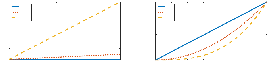
Figure 4: Relative distribution weight

0 20 40 60 80 100 120 140

deposit

100

HANK

L10

L100

0 20 40 60 80 100 120 140

deposit

L10

S10

C10

Notes: This ﬁgure plots the relative weight of dividend obtained by people at diﬀerent wealth level at the

stationary distribution (1 +

). The blue solid lines, red dotted lines, and the yellow dashed lines on

the left(right) column are for the baseline HANK(L10), L10(S10), and L100(C10) models, respectively. The

x-axis is the wealth level, and the y-axis is the relative weight.

wealth distribution when n is bigger. This has the eﬀect of reducing overall inequality. This

implication is illustrated in the left panel of Figure 5, which plots the stationary wealth

distribution from our model under the same dividend distribution rules as the left panel of

Figure 4. From Figure 5, we can see that higher values of n shift more mass in the stationary

distribution to the right, although this mass remains concentrated away from the far-right

tail.

In the right panel of Figure 4, we compare a linear distribution scheme (solid blue line)

to squared and cubic schemes (dotted-red and dashed-orange lines, respectively). While

the endpoints are the same in all cases, more curvature will increase inequality. We show

this result with the right panel of Figure 5. Relative to a linear distribution scheme, more

curvature has the eﬀect of concentrating much more mass near the borrowing constraint,

which has the eﬀect of increasing overall wealth inequality. For example, in both the squared

and cubic speciﬁcations, there are roughly 1.5 times as many households at the peak of the

stationary distribution relative to the linear scheme.

5.2 Inequality Measures

The exact form of the dividend distribution rule has important implications for the model’s

Lorenz curve as well as its Gini coeﬃcient, both of which are important measures of inequality

Figure 5: Stationary distribution

0 20 40 60 80 100

deposit/labor income

0.02

0.04

0.06

0.08

0.1

HANK

L10

L100

0 20 40 60 80 100

deposit/labor income

0.02

0.04

0.06

0.08

0.1

0.12

L10

S10

C10

Notes: This ﬁgure plots the stationary distribution generated by diﬀerent models. The blue solid lines, red

dotted lines, and the yellow dashed lines on the left(right) are for the baseline HANK(L100), L10(S100), and

L100(C100) models, respectively. The x-axis is the ratio between wealth and labor income, and the y-axis

is the density.

Figure 6: Lorenz curve

0 20 40 60 80 100

population percentile

100

deposit percentile

HANK

L10

L100

45 degree line

0 20 40 60 80 100

population percentile

100

deposit percentile

L10

S10

C10

45 degree line

Notes: This ﬁgure plots the Lorenz curve of stationary wealth distribution when the dividends are distributed

according to diﬀerent functions. The blue solid lines, red dotted lines, and the yellow dashed lines on the

left(right) column are for the baseline HANK(L10), L10(S10), and L100(C10) models, respectively, the thin

black solid lines are the 45 degree line. The x-axis is the fraction of population, and the y-axis is the fraction

of wealth.

on which the extant literature has often focused.

Figure 6 plots Lorenz curves for diﬀerent dividend distribution schemes. A Lorenz curve

plots the cumulative fraction of overall wealth against the population percentile. In our

model, household wealth takes the form of deposits. Points along the 45-degree line represent

perfect equality; points below the 45-degree line indicate that wealth is unequally distributed,

with more wealth held by a small fraction of households.

Table 2: Gini coeﬃcient

HANK L10 L100 S10 C10

Gini coeﬀ. 0.44 0.39 0.34 0.48 0.51

Notes: This table reports the Gini coeﬃcients in diﬀerent models.

The left panel plots the Lorenz curves for linear distribution rules. The blue line corre-

sponds to our baseline speciﬁcation (labeled HANK, with equal dividend distribution). The

dotted red curve and the dashed orange curve show the Lorenz curves associated with linear

distribution schemes with larger values of n (10 and 100). Consistent with the shapes of

the stationary distributions, a larger value of n reduces observed inequality and shifts the

Lorenz curves upward. In the right panel, we plot Lorenz Curves conditioning on n = 10,

but for diﬀerent values of ϑ. Here we observe that larger values of ϑ shift the Lorenz curve

down, meaning there is more inequality.

Table 2 corroborates the results depicted graphically in Figure 6 by showing Gini co-

eﬃcients for diﬀerent dividend distribution rules. The Gini coeﬃcient is the ratio of the

area between the 45-degree line and the Lorenz curve to the total area under the 45-degree

line. A larger Gini coeﬃcient indicates higher inequality. Our baseline HANK speciﬁcation

produces a Gini coeﬃcient of 0.44. Focusing on a linear distribution scheme with higher

values of n, the model’s Gini coeﬃcient falls. A squared or cubic speciﬁcation, in contrast,

results in more observed inequality.

5.3 Macro Aggregates

Our analysis above suggests that our model is capable of generating sizable wealth inequality

with alternative dividend distribution rules. However, the question we are interested in is

not whether the model can match moments of the wealth distribution. Rather, the key

question of the paper is whether a model featuring more (or less) inequality matters for the

transmission of QE shocks into aggregate variables. We show in this subsection that there is

little economically meaningful connection between the dividend distribution rule, inequality

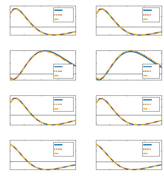
Figure 7: Impulse responses to a QE shock: HANK with diﬀerent distribution

rules

5 10 15 20

0.5

output

HANK

L10

L100

5 10 15 20

0.1

0.2

consumption

HANK

L10

L100

5 10 15 20

-2

investment

HANK

L10

L100

5 10 15 20

0.05

0.1

inflation

HANK

L10

L100

5 10 15 20

0.5

output

L10

S10

C10

5 10 15 20

0.1

0.2

consumption

L10

S10

C10

5 10 15 20

-2

investment

L10

S10

C10

5 10 15 20

0.05

0.1

inflation

L10

S10

C10

Notes: This ﬁgure plots the impulse responses of aggregate variables with linear distribution under a positive

QE shock. The blue solid lines, red dotted lines, and the yellow dashed lines in the left(right) column are

for the baseline HANK(L10), L10(S10), and L100(C10) models, respectively. The x-axis is time, and y-axis

is the percentage change from steady state.

moments, and aggregate eﬀects of QE shocks.

Figure 7 plots impulse responses to a QE shock under diﬀerent dividend distribution

speciﬁcations. The picture is divided into two panels, with responses in the HANK, L10, and

L100 speciﬁcations in the left panel, and responses for the L10, S10, and C10 speciﬁcations

in the right panel. We focus only on responses of output, consumption, investment, and

inﬂation here, but the responses are otherwise generated in the same manner as in Figure 2.

The responses of aggregate variables to a QE shock are remarkably similar under all

speciﬁcations; this means they are all, in turn, very close to the RANK speciﬁcation as well.

There are some small diﬀerences for the response of aggregate consumption, but the inﬂation,

output, and investment responses are almost identical across all speciﬁcations. These results

suggest that the exact form of the dividend distribution rule – though relevant for inequality

moments like the Gini coeﬃcient – is unimportant for the aggregate transmission of a QE

shock. This, in turn, suggests that the literature’s heavy focus on these inequality statistics

may be misplaced, at least to the extent to which one focuses on dynamics of aggregate

variables.

6 Implications of the Macro-Distribution of Wealth

In this section, we investigate how some parameters related to the macro-distribution of

wealth impact our results. In particular, we are interested in how parameters such as the

unemployment rate, the unemployment beneﬁt, the unemployment duration, and households’

risk aversion aﬀect the stationary wealth distribution, and in turn the aggregate transmission

of QE shocks.

6.1 Unemployment Rate

In our baseline calibration, we set the unemployment rate to ﬁve percent. While consistent

with the data, this relatively low unemployment rate means that households face a small

probability of job loss. In this section, we allow a higher unemployment rate, which means

households face more uninsurable income risk, and study its implications for the behavior of

aggregate consumption, and hence other aggregate variables, in response to a QE shock.

Figure 8 plots the stationary wealth distribution in our model with four diﬀerent targets

for the unemployment rate – our baseline speciﬁcation of ﬁve percent, labeled HANK (solid

blue line), 10 percent (dotted red line), 20 percent (dashed orange line), and 40 percent

(dashed purple line). While a 40 percent unemployment rate is clearly unrealistic, it is not

unreasonable compared to labor force non-participation rates. Increasing the unemployment

rates shifts mass in the stationary distribution towards the borrowing constraint.

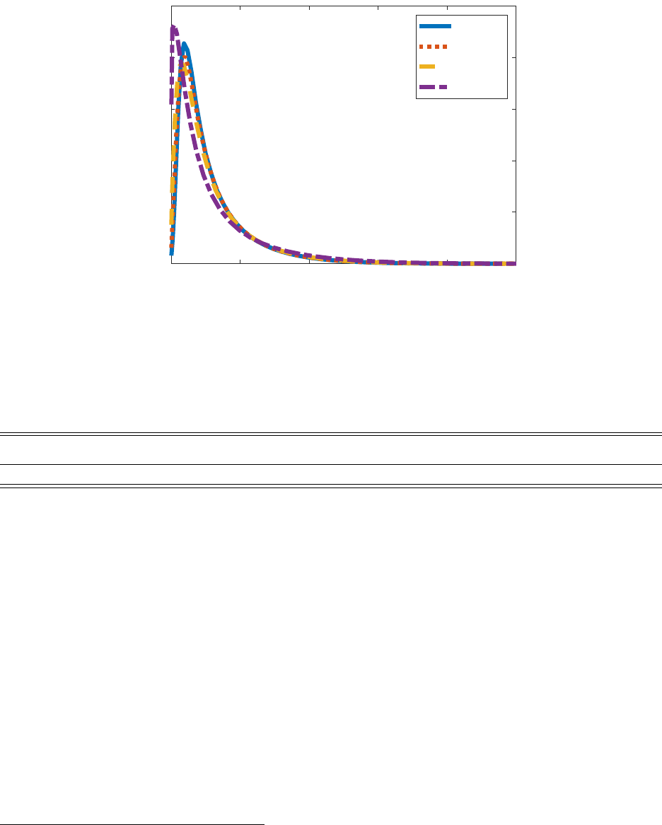
Figure 8: Stationary Distribution: HANK vs. U = 10%, 20% and 40%

0 20 40 60 80 100

deposit/labor income

0.02

0.04

0.06

0.08

0.1

HANK

U=10%

U=20%

U=40%

Notes: This ﬁgure plots the stationary distribution of the population. The blue solid line is for the HANK

model, the red dotted line is for the model with 10% unemployment rate, the yellow dashed line is for the

model with 20% unemployment rate, and the purple dash-dotted line is for the model with 40% unemploy-

ment rate. The x-axis is the ratio between wealth and average steady state labor income, and the y-axis is

the density.

Table 3: Households At and Near the Borrowing Constraint

HANK U = 10% U = 20% U = 40% µ = 30% µ = 50%

7.80 5.81 5.94 19.60 4.76 13.22

Notes: This table reports the percentage of households near the borrowing constraint (deﬁned as having

deposits less than two quarters’ worth of average steady-state labor income) in diﬀerent models.

Table 3 shows the percentage of households located at or near the borrowing constraint in

diﬀerent speciﬁcations of our model. We deﬁne households as near the borrowing constraint

if their accumulated wealth amounts to less than two quarters’ worth of average steady-state

labor income. In our baseline HANK model, just under 8 percent of households are near

the borrowing constraint. When the unemployment rate is 40 percent, nearly 20 percent of

households have fewer than two quarters’ worth of labor income saved. It appears as though

fewer households are located near the constraint for intermediate values of unemployment

of 10 and 20 percent. This is an artifact of the way we discretize the deposit grids.

The

Since lower unemployment results in higher average labor income, fewer deposit grid points satisfy the

condition that deposits are less than two quarters’ steady-state labor income.

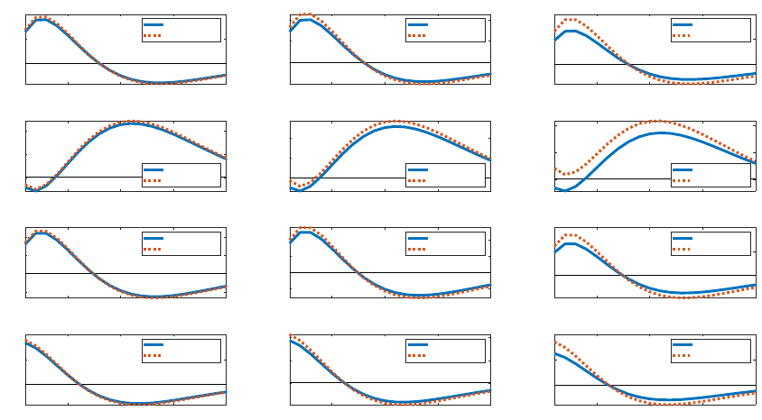
Figure 9: Impulse responses to a QE shock: HANK vs. RANK for U = 10%, 20%,

and 40%

5 10 15 20

0.5

output

RANK--U=10%

HANK--U=10%

5 10 15 20

0.1

0.2

consumption

RANK--U=10%

HANK--U=10%

5 10 15 20

-2

investment

RANK--U=10%

HANK--U=10%

5 10 15 20

0.05

0.1

inflation

RANK--U=10%

HANK--U=10%

5 10 15 20

-0.5

0.5

output

RANK--U=20%

HANK--U=20%

5 10 15 20

0.1

0.2

consumption

RANK--U=20%

HANK--U=20%

5 10 15 20

-2

investment

RANK--U=20%

HANK--U=20%

5 10 15 20

0.05

0.1

inflation

RANK--U=20%

HANK--U=20%

5 10 15 20

output

RANK--U=40%

HANK--U=40%

5 10 15 20

0.2

0.4

consumption

RANK--U=40%

HANK--U=40%

5 10 15 20

investment

RANK--U=40%

HANK--U=40%

5 10 15 20

0.1

0.2

inflation

RANK--U=40%

HANK--U=40%

Notes: This ﬁgure plots the impulse responses of aggregate variables under a 4% QE shock. The blue

solid lines and red dotted lines on the left/middle/right column are for the HANK and RANK models with

10%/20%/40% unemployment rate, respectively. The x-axis is time, and the y-axis is the percentage change

from steady state.

extreme value of 40 percent unemployment gives a clearer sense of how the wealth distribution

varies with the unemployment rate. Note further, these numbers tend to underestimate

the true fraction of households that are located near the borrowing constraint because poor

people tend to work more and hence have a higher steady-state income than richer households

via a wealth channel, but we are deﬁning being near the borrowing constraint based on

average labor income, not the income of individual households. This makes the denominator

smaller and the overall wealth/income larger.

Figure 9 plots impulse response to a QE shock in these scenarios. The left/middle/right

panel considers an unemployment target of 10/20/40 percent. Solid blue lines refer to re-

sponses in a RANK version of our model, calibrated to have a comparable steady state labor

input as the corresponding HANK model. Dotted red lines are impulse responses in a HANK

model. Compared to a RANK model, aggregate variables react more the higher is the unem-

ployment rate. These diﬀerences are small and mostly not visible for a 10 percent and even

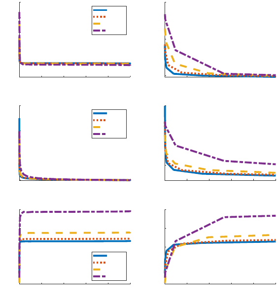
Figure 10: First period individual responses to a QE shock: HANK vs. U = 10%,

20%, and 40%

0 20 40 60 80 100

-0.5

0.5

1.5

consumption

HANK

U=10%

U=20%

U=40%

0 20 40 60 80 100

deposit

HANK

U=10%

U=20%

U=40%

0 20 40 60 80 100

deposit percentile

-0.5

0.5

1.5

labor

HANK

U=10%

U=20%

U=40%

0 0.2 0.4 0.6 0.8 1

0.5

1.5

consumption

0 0.2 0.4 0.6 0.8 1

deposit

0 0.2 0.4 0.6 0.8 1

deposit percentile

-0.5

0.5

1.5

labor

Notes: This ﬁgure plots the impulse responses of (employed) individual decision variables (consumption,

deposits, and labor supply) in the period when a 4% positive QE shock hits. The blue solid lines, red dotted

lines, yellow dashed lines, and purple dash-dotted lines are for the baseline HANK model and the models

with U = 10%, U = 20%, and U = 40%, respectively. The x-axis is the wealth fraction from poor to rich,

and the y-axis is the percentage change from steady state. The left panel plots ﬁrst-period responses across

the full wealth distribution, while the right panel zooms in on the bottom one percent.

a 20 percent unemployment target. There are somewhat more meaningful diﬀerences when

we target unemployment of 40 percent. Consumption rises, rather than falls, with output

and investment reacting about 20 percent more on impact to an expansionary QE shock

compared to a RANK model. Still, the responses with this extreme value of unemployment

are nevertheless qualitatively similar to the RANK speciﬁcation as well as to our benchmark

HANK model.

To provide some intuition, Figure 10 plots the ﬁrst-period individual choice variable

responses to a QE shock as a function of wealth. The ﬁgure is analogous to Figure 3, but

compares HANK responses with diﬀerent unemployment rates. The main diﬀerences are for

Figure 11: Stationary Distribution: HANK vs µ = 30% and 50%

0 20 40 60 80 100

deposit/labor income

0.02

0.04

0.06

0.08

0.1

HANK

=30%

=50%

Notes: This ﬁgure plots the stationary distribution of the population. The blue solid lines are for the HANK

model, the red dotted lines are for the model with 30% unemployment beneﬁts, and the yellow dashed lines

are for the model with 50% unemployment beneﬁts. The x-axis is the ratio between wealth and labor income,

and the y-axis is the density.

the poorest households, who increase their consumption and savings, and decrease labor,

by more the higher is the unemployment rate. It remains the case that households located

further from the borrowing constraint behave similarly with respect to consumption and

saving choices across diﬀerent speciﬁcations, and in turn, similarly to the representative

agent counterpart from a RANK speciﬁcation.

6.2 Unemployment Beneﬁt

We next consider the role played by the unemployment beneﬁt, µ in our model. We consider

both a smaller (µ = 0.30) and larger (µ = 0.50) value of this parameter compared to our

benchmark speciﬁcation (µ = 0.40). Figure 11 plots the stationary distributions of wealth

for these three diﬀerent values of the unemployment beneﬁt. The bigger is µ, the more

mass is concentrated in the left tail near the borrowing constraint. The reason for this is

straightforward – with a bigger unemployment beneﬁt, the cost of unemployment is smaller,

and households consequently have less incentive to self-insure against unemployment by

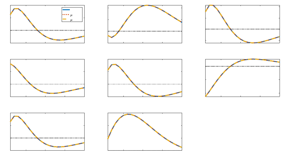
Figure 12: Impulse responses to a QE shock: HANK vs. µ = 30% and 50%

5 10 15 20

-0.5

0.5

output

HANK

=30%

=50%

5 10 15 20

-0.1

0.1

0.2

consumption

5 10 15 20

-2

investment

5 10 15 20

-0.05

0.05

0.1

inflation

5 10 15 20

-0.05

0.05

0.1

policy rate

5 10 15 20

-0.2

-0.1

corp. bond spread

5 10 15 20

-0.5

0.5

labor

5 10 15 20

0.5

1.5

deposit

Notes: This ﬁgure plots the impulse responses of aggregate variables under a 4% QE shock. The blue solid

lines are for the HANK model, the red dotted lines are for the model with 30% unemployment beneﬁts, and

the yellow dashed lines are for the model with 50% unemployment beneﬁts. X-axis is time in quarters, and

Y-axis is the percentage change from steady state.

saving. We see this channel at play in the right columns of Table 3, which show that with a

higher value of µ, a larger percentage of households are located near the borrowing constraint.

Figure 12 plots the impulse responses of aggregate variables to a QE shock with these

diﬀerent values of the unemployment beneﬁt. The responses with µ = 0.30 or µ = 0.50 are

virtually identical to the responses in our benchmark HANK speciﬁcation.

6.3 Unemployment Duration

The duration of unemployment spells, governed in our model by the parameter p, is another

parameter of interest. In our benchmark model, we set this parameter to p = 1/2, implying

an average duration of unemployment spells of two quarters. We consider now a value of

p = 9/10, which implies a typical duration of unemployment of 10 quarters. The model is

re-parameterized with this new value of p to still target our benchmark unemployment rate

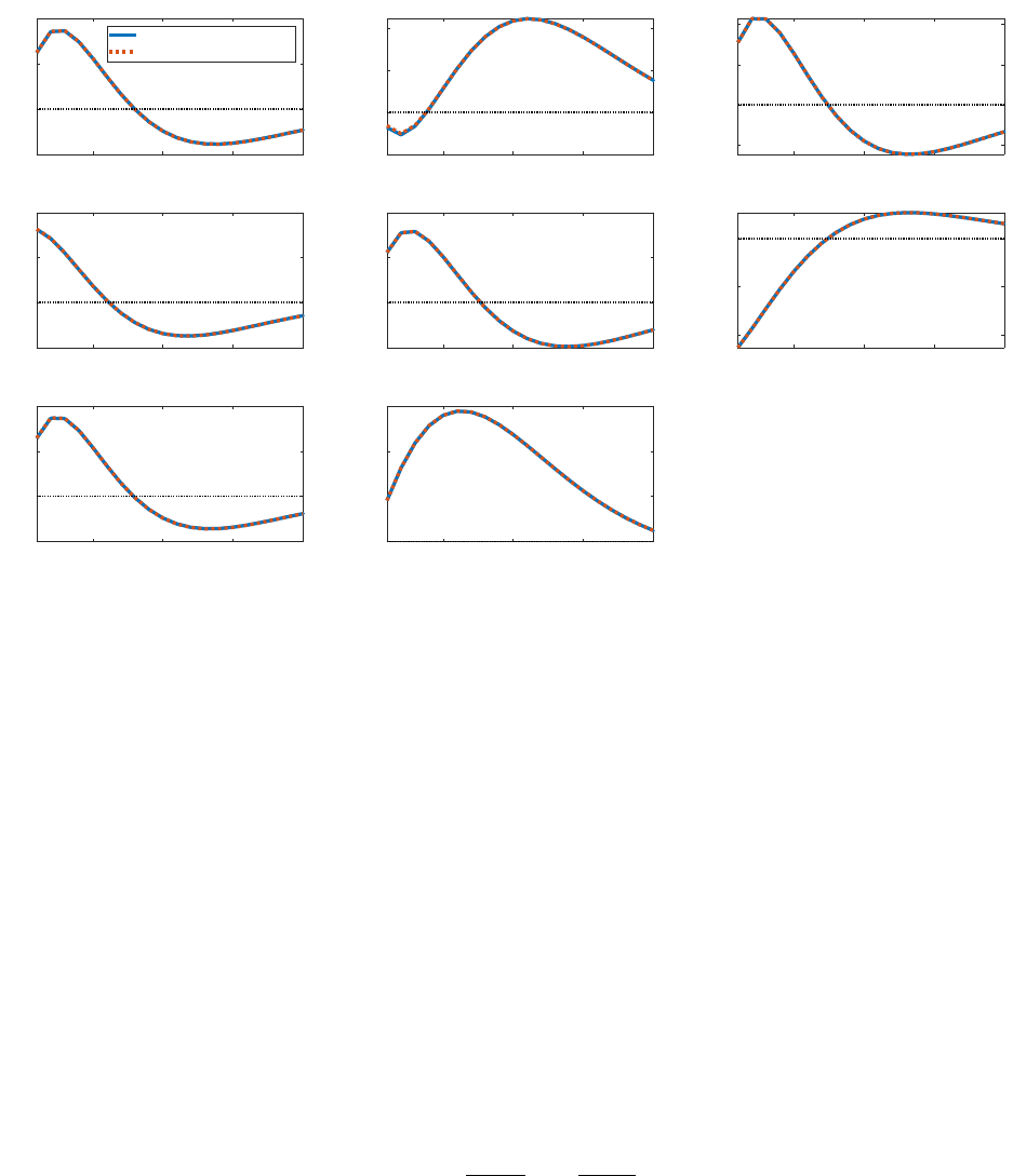
Figure 13: Impulse responses to a QE shock: unemployment duration = 2 vs. 10

quarters

5 10 15 20

-0.5

0.5

output

Unemployment duration=2

Unemployment duration=10

5 10 15 20

-0.1

0.1

0.2

consumption

5 10 15 20

-2

investment

5 10 15 20

-0.05

0.05

0.1

inflation

5 10 15 20

-0.05

0.05

0.1

policy rate

5 10 15 20

-0.2

-0.1

corp. bond spread

5 10 15 20

-0.5

0.5

labor

5 10 15 20

0.5

1.5

deposit

Notes: This ﬁgure plots the impulse responses of aggregate variables under a 4% QE shock. The blue solid

lines are for the RANK model, and the red dashed lines are for the HANK model. X-axis is time in quarters,

and Y-axis is the percentage change from steady state.

of ﬁve percent. Figure 13 plots aggregate responses to a QE shock for both our baseline

HANK speciﬁcation as well as this new speciﬁcation with a lower value of p. The aggregate

impulse responses are virtually identical.

6.4 Risk Aversion

Finally, we investigate the role played by households’ degree of risk aversion. Instead of

assuming log utility over consumption as in (2.1), we allow for a more general isoelastic

utility function, with lifetime ﬂow utility now given by:

∞

t=0

1−σ

i,t

1 − σ

− χ

1+η

j,t

1 + η

where σ measures the coeﬃcient of relative risk aversion. Log utility is a special case with

σ = 1.

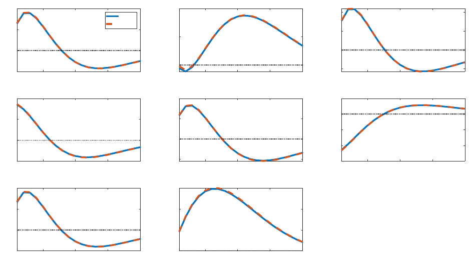
Figure 14: Impulse responses to a QE shock: RANK vs. HANK for CRRA utility

5 10 15 20

-0.5

0.5

output

RANK

HANK

5 10 15 20

0.05

0.1

consumption

5 10 15 20

-2

investment

5 10 15 20

-0.05

0.05

0.1

inflation

5 10 15 20

-0.05

0.05

0.1

policy rate

5 10 15 20

-0.3

-0.2

-0.1

0.1

corp. bond spread

5 10 15 20

-0.5

0.5

labor

5 10 15 20

0.5

1.5

deposit

Notes: This ﬁgure plots the impulse responses of aggregate variables under a 4% QE shock. The blue solid

lines are for the RANK model, and the red dashed lines are for the HANK model. X-axis is time in quarters,

and Y-axis is the percentage change from steady state.

We consider a higher value of σ = 3, implying substantially more risk aversion than in

the case of log utility. Figure 14 plots impulse responses for a RANK version of our model

with σ = 3 (solid blue) and the HANK version with the same risk aversion (dashed red).

There is practically no diﬀerence between the two speciﬁcations.

7 Conclusion

We developed a quantitative DSGE model to study the aggregate implications of central bank

asset purchases when there is substantial household wealth heterogeneity. The ﬁnancial

and production sides of the model are similar to Sims and Wu (2021a), which features

constrained ﬁnancial intermediaries and scope for QE to matter. We model households

similarly to Krusell and Smith (1998): they are heterogeneous with respect to wealth, face

uninsurable unemployment risk, and are subject to a borrowing constraint. Diﬀerent from

them, households endogenously choose labor supply. We developed a solution method that

is compatible with Dynare and uses perturbation methods to solve and simulate the model.

We ﬁnd that the aggregate responses to central bank asset purchases are very similar in

a HANK speciﬁcation compared to a RANK version of the model. We consider alternative

assumptions about the micro- and macro-distributions of wealth. For the former, we vary

how dividends are distributed across households. While diﬀerent dividend distribution rules

can generate diﬀerent amounts of wealth inequality based on popular metrics, they have

little discernible impact on how aggregate variables like output react to a QE shock. For the

latter, we examine how the unemployment rate, the unemployment beneﬁt, the duration of

unemployment, and the degree of relative risk aversion impact the aggregate transmission of

QE shocks. For reasonable values of macro parameters, we ﬁnd no discernible diﬀerences in

the impact of QE shocks between HANK and RANK models. We conclude that a RANK

speciﬁcation may provide an adequate approximation for understanding the aggregate im-

plications of QE.

References

Acharya, Sushant and Keshav Dogra, “Understanding HANK: Insights From a

PRANK,” Econometrica, 2020, 88 (3), 1113–1158.

Algan, Yann, Olivier Allais, and Wouter J. Den Haan, “Solving heterogeneous-agent

models with parameterized cross-sectional distributions,” Journal of Economic Dynamics

and Control, 2008, 32 (3), 875 – 908.

Alves, Felipe, Greg Kaplan, Benjamin Moll, and Giovanni Violante, “A Further

Look at the Propagation of Monetary Policy Shocks in HANK,” Journal of Money, Credit

and Banking, 2020, 52 (S2), 521–559.

Auclert, Adrien, “Monetary Policy and the Redistribution Channel,” American Economic

Review, June 2019, 109 (6), 2333–67.

Cui, Wei and Vincent Sterk, “Quantitative easing with heterogeneous agents,” Journal

of Monetary Economics, October 2021, 123, 68–90.

Debortoli, Davide and Jordi Gali, “Idiosyncratic Income Risk and Aggregate Fluctua-

tions,” 2022. NBER Working Paper 29704.

Gertler, Mark and Peter Karadi, “A Model of Unconventional Monetary Policy,” Jour-

nal of Monetary Economics, 2011, pp. 17–34.

and , “QE 1 vs. 2 vs. 3...: A Framework for Analyzing Large-Scale Asset Purchases as

a Monetary Policy Tool,” International Journal of Central Banking, 2013, 9(S1), 5–53.

Judd, Kenneth L., Numerical Methods in Economics, Vol. 1 of MIT Press Books, The

MIT Press, December 1998.

Kaplan, Greg, Benjamin Moll, and Giovanni L. Violante, “Monetary Policy Accord-

ing to HANK,” American Economic Review, March 2018, 108 (3), 697–743.

Krusell, Per and Anthony A. Smith Jr., “Income and wealth heterogeneity in the

macroeconomy,” Journal of Political Economy, 1998, 106 (5), 867–896.

McKay, Alisdair, Emi Nakamura, and J´on Steinsson, “The Power of Forward Guid-

ance Revisited,” American Economic Review, October 2016, 106 (10), 3133–58.

Ravn, Morten O and Vincent Sterk, “Macroeconomic Fluctuations with HANK &

SAM: an Analytical Approach,” Journal of the European Economic Association, 06 2020,

19 (2), 1162–1202.

Reiter, Michael, “Solving heterogeneous-agent models by projection and perturbation,”

Journal of Economic Dynamics and Control, 2009, 33, 649–665.

Shimer, Robert, “The Cyclical Behavior of Equilibrium Unemployment and Vacancies,”

American Economic Review, March 2005, 95 (1), 25–49.

Sims, Eric and Jing Cynthia Wu, “Are QE and Conventional Monetary Policy Substi-

tutable?,” International Journal of Central Banking, 2020, 16 (1), 195–230.

and , “Evaluating Central Banks’ Tool Kit: Past, Present, and Future,” Journal of

Monetary Economics, 2021, 185, 135–160.

and , “Wall Street QE vs. Main Street Lending,” 2021. NBER Working Paper No.

27295.

, , and Ji Zhang, “The Four Equation New Keynesian Model,” Review of Economics

and Statistics, forthcoming.

Taylor, John B., “Discretion versus Policy Rules in Practice,” Carnegie-Rochester Con-

ference Series on Public Policy, 1993, 39, 195–214.

Winberry, Thomas, “A method for solving and estimating heterogeneous agent macro

models,” Quantitative Economics, 2018, 9 (3), 1123–1151.

Woodford, Michael, “Fiscal requirements for price stability,” JMCB, August 2001, 33 (3),

669–728.

Young, Eric R., “Solving the incomplete markets model with aggregate uncertainty us-

ing the Krusell–Smith algorithm and non-stochastic simulations,” Journal of Economic

Dynamics and Control, 2010, 34 (1), 36 – 41.

A Model Details

This appendix contains details from the model discussed in Section 2.

A.1 Labor Market

Labor unions, indexed by h ∈ [0, 1] purchase labor from households at price M RS

, repackage it into L

d,t

(h),

and sell it to a representative labor contractor. A representative labor contractor combines diﬀerentiated

labor into ﬁnal labor used in production, via CES technology with elasticity ε

. The demand curve each

labor union faces is

d,t

(h) =



(h)



−ε

d,t

(A.1)

(h) is the wage paid for union h’s labor and W

is the aggregate wage, which satisﬁes

1−ϵ

(h)

1−ϵ

dh (A.2)

Labor unions are subject to a Calvo-type nominal rigidity. Each period, a union may re-optimize its

wage with probability 1 − ϕ

with ϕ

∈ [0, 1]. Non-reoptimized wages are indexed to lagged inﬂation at

∈ [0, 1]. A labor union chooses a wage to maximize the present discounted value of real proﬁts:

max

(h)

∞

j=0

t,t+j



t+j−1

t−1



(1−ϵ

)γ

(h)

1−ϵ

t−1

t+j

d,t+j

−

mrs

t+j



t+j−1

t−1



−ϵ

(h)

−ϵ

t+j

d,t+j

(A.3)

where Λ

t,t+j

= Λ

t,t+1

· · · Λ

t+j−1,t+j

The ﬁrst order condition is

(ϵ

− 1)W

(h)

−ϵ

∞

j=0

t,t+j



t+j−1

t−1



(1−ϵ

)γ

−1

t+j

d,t+j

(h)

−ϵ

−1

∞

j=0

t,t+j

mrs

t+j



t+j−1

t−1



−ϵ

t+j

d,t+j

The reset wage is the same across all labor unions. Hence, drop the h index, and the optimal price W

∗

can

be written as:

∗

− 1

1,t

2,t

where F

1,t

and F

2,t

are recursive representations of the inﬁnite sums above:

1,t

= mrs

d,t

+ ϕ

t,t+1

−ϵ

1,t+1

2,t

= P

−1

d,t

+ ϕ

t,t+1

(1−ϵ

)γ

2,t+1

Written in real terms, w

∗

= W

∗

, it satisﬁes:

∗

− 1

1,t

2,t

(A.4)

1,t

= mrs

d,t

+ ϕ

t,t+1



t+1



1,t+1

(A.5)

2,t

= w

d,t

+ ϕ

t,t+1



t+1



−1

2,t+1

(A.6)

where w

= W

is the aggregate real wage from (A.2), and f

1,t

= F

1,t

and f

2,t

= F

2,t

−1

Aggregation Integrate (A.1) across h, noting that

d,t

(h)dh = L

. Using the demand function for

a union’s labor, (A.1), yields

= L

d,t

(A.7)

where v

is a measure of wage dispersion:



(h)



−ϵ

Note that this can be written in terms of real wages since it is a ratio. Because of properties of Calvo

wage-setting, we can write this as

= (1 − ϕ

)



∗



−ϵ

1−ϕ



t−1

(h)



−ϵ

= (1 − ϕ

)



∗



−ϵ

+ Π

−γ

t−1

−ϵ

t−1

1−ϕ



t−1

(h)

t−1



−ϵ

which may be written as

= (1 − ϕ

)



∗



−ϵ

+ ϕ

−γ

t−1

−ϵ

t−1

Expressing this in real terms gives

= (1 − ϕ

)



∗



−ϵ

+ ϕ



t−1





t−1



t−1

(A.8)

From (A.2), we have

1−ϵ

= (1 − ϕ

) (W

∗

)

1−ϵ

1−ϕ



t−1

(h)



1−ϵ

Via a law of large numbers, this is

1−ϵ

= (1 − ϕ

) (W

∗

)

1−ϵ

+ Π

(1−ϵ

)

t−1

1−ϵ

t−1

Dividing both sides by P

1−ϵ

gives

1−ϵ

= (1 − ϕ

) (w

∗

)

1−ϵ

+ ϕ

(1−ϵ

)

t−1

−1

1−ϵ

t−1

(A.9)

A.2 Capital Producers

A representative capital producer transfers raw investment goods I

into new capital

via:



1 − S



t−1



(A.10)

where S (I

t−1

) =

t−1

− 1)

is the investment adjustment cost.

The capital producer sells new capital to wholesale ﬁrms, and earns real proﬁt in period t:

div

k,t

= p



1 − S



t−1



− I

(A.11)

where p

is the real price of new capital. The object of a capital producer is to maximize the present value

of proﬁt:

max

∞

j=0

t,t+j





1 − S



t+j

t+j−1



t+j

− I

t+j



The ﬁrst order condition is

1 = p



1 − S



t−1



− S

′



t−1



t−1



+ E

t,t+1

t+1

′



t+1



t+1



(A.12)

A.3 Output

The ﬁnal output good, Y

, is a CES aggregate of retail outputs with elasticity of substitution ϵ

> 1. Proﬁt

maximization by the ﬁnal good producer generates a demand curve for each retail output and an expression

for the aggregate price index:

(f) =



(f)



−ϵ

. (A.13)

The price of the ﬁnal goods, P

, satisﬁes:

1−ϵ

(f)

1−ϵ

df. (A.14)

Each period, a retailer faces a constant probability, 1 − ϕ

, of being able to adjust its price. Consider

the problem of a retailer given the opportunity to adjust in period t. When it sets a price, it must take into

account that the price chosen in t will still be in eﬀect in period t + j with probability ϕ

. Indexation to

lagged inﬂation means that an unupdated price in period t + j will be: P

(f)



t+j−1

t−1



. When choosing a

price, the retailer maximizes the present discounted value of real proﬁts returned to the household, where

discounting is by the household’s stochastic discount factor augmented by the probability of non-adjustment:

max

(f)

∞

j=0

t,t+j

(f)

1−ϵ



t+j−1

t−1



(1−ϵ

)γ

−1

t+j

− P

m,t+j

(f)

−ϵ



t+j−1

t−1



−ϵ

−1

t+j

The ﬁrst order condition is

(ϵ

− 1)P

(f)

−ϵ

∞

j=0

t,t+j



t+j−1

t−1



(1−ϵ

)γ

−1

t+j

(f)

−ϵ

−1

∞

j=0

t,t+j

m,t+j



t+j−1

t−1



−ϵ

t+j

Deﬁne variables:

1,t

∞

j=0

(ϕ

β)

t+j

m,t+j



t+j−1

t−1



−ϵ

t+j

2,t

∞

j=0

(ϕ

β)

t+j



t+j−1

t−1



(1−ϵ

)γ

−1

t+j

These can be written recursively as:

1,t

= p

m,t

+ ϕ

t,t+1

−ϵ

1,t+1

2,t

= P

−1

+ ϕ

t,t+1

(1−ϵ

)γ

2,t+1

Note, all retailers set the same price. We call this reset price P

∗

. Hence, the ﬁrst order condition can be

written as

∗

− 1

1,t

2,t

Deﬁning x

1,t

= X

1,t

, x

2,t

= X

2,t

−1

, and p

∗

= P

∗

gives

∗

− 1

1,t

2,t

(A.15)

1,t

= p

m,t

+ ϕ

t,t+1



t+1



1,t+1

(A.16)

2,t

= Y

+ ϕ

t,t+1



t+1



−1

2,t+1

(A.17)

where p

m,t

Aggregation Integrate the demand for retail output, (A.13), across retailers, noting that Y

(f) =

m,t

(f),

m,t

(f)df = Y

m,t

, where Y

m,t

is wholesale output. This yields

= Y

m,t

(A.18)

where



(f)



−ϵ

This is a measure of price dispersion. Using properties of Calvo pricing with indexation to lagged inﬂation

yields:

= (1 − ϕ

) (p

∗

)

−ϵ

1−ϕ

t−1

(f)

−ϵ

= (1 − ϕ

) (p

∗

)

−ϵ

+ Π

−γ

t−1

−ϵ

t−1

1−ϕ



t−1

(f)

t−1



−ϵ

Via a law of large numbers, this reduces to

= (1 − ϕ

) (p

∗

)

−ϵ

+ ϕ

t−1

(A.19)

Similarly, the aggregate price index, (A.14), may be written as:

1−ϵ

= (1 − ϕ

) (P

∗

)

1−ϵ

1−ϕ

(1−ϵ

)

t−1

(f)

1−ϵ

= (1 − ϕ

) (P

∗

)

1−ϵ

+ ϕ

(1−ϵ

)

t−1

1−ϵ

t−1

Divide both sides by P

1−ϵ

to obtain

1 = (1 − ϕ

) (p

∗

)

1−ϵ

+ ϕ

(1−ϵ

)

t−1

−1

(A.20)

The representative wholesale ﬁrm produces output according to a Cobb-Douglas technology:

m,t

= A

)

1−α

d,t

(A.21)

m,t

is ﬂow output, u

is the capital utilization rate, and L

d,t

is labor input. 0 < α < 1 is the exponent on

capital services in the production function. A

is an exogenous productivity variable that obeys an exogenous

stochastic process. K

is the stock of physical capital, which the ﬁrm owns. Physical capital accumulates

according to a standard law of motion:

t+1

+ (1 − δ(u

))K

(A.22)

where δ (u

) = δ

+δ

− 1)+

− 1)

is the capital depreciation rate and depends on capital utilization.

The wholesale ﬁrm must issue perpetual bonds to ﬁnance the purchase of new physical capital,

Diﬀerent than them, we only require the ﬁrm to ﬁnance a constant fraction, ψ ∈ [0, 1], of investment, not

the entirety. This gives rise to a “loan in advance constraint” of the form:

ψP

≤ Q

m,t

= Q

m,t

− κF

m,t−1

) , (A.23)

where P

is the price at which the wholesale ﬁrm purchases new physical capital.

The wholesale ﬁrm hires labor in a competitive spot market at nominal wage W

. Its nominal dividend

DIV

m,t

= P

m,t

1−α

d,t

− W

d,t

− P

− F

m,t−1

+ Q

m,t

− κF

m,t−1

) (A.24)

The ﬁrm maximizes the present discounted value of real dividends, where discounting is by the stochastic

discount factor of households. The ﬁrst order conditions are

= (1 − α)p

m,t

−α

d,t

(A.25)

1,t

′

) = αp

m,t

)

α−1

1−α

d,t

(A.26)

1,t

= E

t,t+1

αp

m,t+1

t+1

α−1

t+1

1−α

d,t+1

+ (1 − δ(u

))p

t+1

1,t+1

(A.27)

2,t

= E

t,t+1

−1

t+1

[1 + κQ

t+1

2,t+1

] (A.28)

1,t

− 1

2,t

− 1

= ψ (A.29)

= W

is the real wage, p

m,t

= P

m,t

is the relative price of wholesale output, and p

= P

is the

relative price of new capital. (A.25) is the standard static ﬁrst order condition for labor demand. M

1,t

is one

plus the product of ψ with the multiplier on the constraint that ﬁrms must issue bonds to ﬁnance investment,

(A.23), while M

2,t

is simply one plus the multiplier on the constraint. (A.26) is the ﬁrst-order condition for

capital utilization. (A.27) and (A.28) are optimality conditions for capital and bonds, respectively. If the

constraint did not bind, then M

1,t

= M

2,t

= 1 and (A.27) - (A.28) would reduce to standard asset pricing

conditions. M

1,t

serves as an endogenous “investment wedge” and M

2,t

can be thought of as a “ﬁnancial

wedge.” These wedges distort the standard asset pricing decisions and ﬂuctuations in these wedges are the

mechanism through which QE type policies transmit to the real economy.

A.4 Exogenous Processes and Aggregation

Aggregate productivity, A

, and government spending, G

follow AR(1) processes in the log:

ln A

= ρ

ln A

t−1

+ s

A,t

, (A.30)

ln G

= (1 − ρ

) ln G + ρ

ln G

t−1

+ s

G,t

. (A.31)

Autoregressive parameters are restricted to lie between zero and one, and shocks are drawn from standard

normal distributions, with s

, and s

denoting standard deviations. G is the non-stochastic steady state

value of government spending. The non-stochastic steady state value of labor productivity is normalized to

unity.

The exogenous process for central bank holdings of private bonds is given in (2.28). There is a similar

law of motion for central bank holdings of government bonds:

ln b

cb,t

= (1 − ρ

+ ρ

ln b

cb,t−1

+ σ

b,t

. (A.32)

There are therefore ﬁve exogenous shocks in the model: productivity (ϵ

A,t

), government spending (ϵ

G,t

monetary policy (ϵ

r,t

), private QE (ϵ

f,t

), and public QE (ϵ

b,t

Privately-issued and government-issued bonds must be held by either ﬁnancial intermediaries or the

central bank. In real terms, the bond market-clearing conditions are:

m,t

= f

+ f

cb,t

(A.33)

= b

+ b

cb,t

, (A.34)

where f

i,t

and b

i,t

Aggregated across intermediaries, and written in real terms, the aggregate ﬁnancial intermediary balance

sheet condition is:

+ Q

B,t

+ re

= d

+ n

. (A.35)

The aggregate dynamics of intermediary net worth are given by:

= σΠ

−1

− R

t−1

+ (R

− R

t−1

B,t−1

t−1

+ (R

t−1

− R

t−1

)re

t−1

+ R

t−1

+ X (A.36)

Similarly, aggregating the endogenous leverage constraint across intermediaries yields:

+ ∆Q

B,t

≤ ϕ

(A.37)

The total dividends from the retail ﬁrms, wholesale ﬁrm, capital producer, labor union, and ﬁnancial

intermediaries amount to

div

= Y

− mrs

− I

+ Q



m,t

− κ

m,t−1



−

m,t−1

1 − σ

− X). (A.38)

The aggregate resource constraint is standard:

= C

+ I

+ G

(A.39)

B Approximating Individual Policy Functions

For the Chebyshev polynomials in (3.1), ξ(d) = 2

d−d

− 1 transforms the interval d ∈ (d,

d) to (−1, 1), and

the Chebyshev polynomials are deﬁned as following:

(x) = cos(n arccos x) (B.1)

The algorithm aims to ﬁt a set of nodes {d

}

m=1

with an N order polynomial, where M = N + 1. The

Chebyshev nodes deﬁned on (−1, 1) are

= − cos



2m − 1



. (B.2)

Adjust nodes to (d,

d) interval:

= (x

+ 1)



d − d



+ d. (B.3)

The policy functions can be solved jointly using (3.2) - (3.4).

For the individual d

t−1

= d

, the right hand side of (3.1) can be expressed as



t+1

−1

t+1



= E





t+1

p(ε

t+1

|ε

t+1

t−1

= d

, ε

), ε

t+1

)

−1





(B.4)

The next step is to compute the right hand side of (B.4), which requires c

t+1

. With d

t−1

, ε

) solved using

(3.2) - (3.4), we can compute conditional expectation next period T(ε

t+1

, d

) by shifting (3.1) one period

forward. Then, we can solve c

t+1

by shifting the system in (3.2) - (3.4) one period forward. Combining (3.1),

(3.1), and (B.4), we have M × 2 equations for M × 2 variables θ

n,t

(ε

n=0

n,t

(ε

(ξ(d

)) = log E





t+1

p(ε

t+1

|ε

t+1

(ε

t+1

, ε

, d

t−1

= d

)

−1





(B.5)

Note, θ

n,t

(ε

) and θ

n,t+1

(ε

t+1

) also enter the right hand side via c

t+1

C Equilibrium conditions

Our algorithm uses Dynare to solve the system of equations listed below.

C.1 Individual Households and Their Distribution

Chebyshev coeﬃcients: M × 2 equations in (B.5) for M × 2 variables θ

n,t

(ε

) for m = 1, ..., M.

Individual decisions: (3.2) - (3.4) for d

, ε

), l

, ε

), c

, ε

) for m = 0, ..., M. These are

(M + 1) × 2 × 3 equations.

Dynamics of the cross sectional distribution: (3.5) for p(d

= d

, ε

t+1

) for m = 0, ..., M , (M + 1) × 2

equations for (M + 1) × 2 probabilities.

C.2 Aggregate Variables

Aggregate deposit and labor (2 equations):

t−1

m=0

p(d

t−1

= d

, ε

) (C.1)

m=0

(ε

, d

t−1

= d

)p(d

t−1

= d

, ε

). (C.2)

Equations for aggregate variables in diﬀerent sectors (31 equations):

Stochastic discount factor: (2.13).

Labor market (3 equations): (A.4) - (A.6).

Production (13 equations): capital producers (A.10) and (A.12), wholesale ﬁrms (A.21) - (A.23) and

(A.25) - (A.29), retailers (A.15) - (A.17).

Financial intermediaries (10 equations): (2.11), (2.12), (2.16) - (2.20), (A.35) - (A.37).

Fiscal authority, central bank, and monetary policy (4 equation): (2.24) - (2.27).

Aggregation (14 equations):

Exogenous processes (4 equations): (2.28), (A.30) - (A.32).

Bond market clearing conditions (2 equations): (A.33) and (A.34).

Aggregation for retailers and labor market (6 equations): (A.18) - (A.20), (A.7) - (A.9).

Dividend and aggregate resource constraint (2 equations): (A.38) and (A.39).

These are 47 equations for 47 variables

, L

, d

, R

, Q

, Ω

, Π

, λ

, ϕ

, re

, n

, C

, w

, p

∗

, x

1,t

2,t

, p

m,t

, Y

m,t

, I

, p

, f

m,t

, M

1,t

, M

2,t

, f

cb,t

, A

, f

, v

, R

, Q

B,t

, G

, T

cb,t

, b

cb,t

, T

, div

, Λ

t−1,t

, mrs

d,t

, w

∗

, f

1,t

, f

2,t

, v

, u

D Solving for the Stationary Equilibrium

(Step 1) Given aggregate deposit and labor supply d, L, we compute steady states for all aggregate vari-

ables.

(Step 2) Solve for the steady state of the Chebyshev coeﬃcients ϑ(ε) = [θ

(ε), ..., θ

(ε)] that approximate

the conditional expectation function. We use the Chebyshev grid d

for m = 1, ..., M, where d

computed using (B.3).

(Step 2.1) Compute the Chebyshev polynomial T

(ξ(d

)) using (B.1).

(Step 2.2) Initialization

(Step 2.2.1) Initialize by assuming d

= d

t−1

= d

, and l =

l, then we can solve consumption

(0)

(ε, d

) using (3.4).

(Step 2.2.2) Compute the right hand side of (B.5) using c

(0)

(ε, d

) from the previous step.

(Step 2.2.3) For each ε, we have a system of M linear equations in (B.5). We can use them

to solve M unknowns in ϑ(ε), and call it ϑ

(0)

(ε). The value of the equation computed

in the previous step is T(d

, ϑ

(0)

(ε)).

(Step 2.3) This step outlines how we update from ϑ

(j)

(ε) to ϑ

(j+1)

(ε). Repeat this step until

(j+1)

(ε) − ϑ

(j)

(ε) is within a speciﬁed tolerance, and call it ϑ(ε) = ϑ

(j+1)

(ε).

(Step 2.3.1) With ϑ

(j)

(ε

) = ϑ

(j)

(ε), we have computed the conditional expectation T(d

t−1

, ϑ

(j)

(ε

)) from the previous iteration.

(Step 2.3.2) Compute current period deposit d

(ε

, d

t−1

= d

), consumption c

(ε

, d

t−1

), and labor supply l

(ε

, d

t−1

= d

) using (3.2) - (3.4) with T(d

t−1

= d

, ϑ

(j)

(ε

)).

Instead of solving a system of equations with kinks, we implement this step as follows:

Assume the borrowing constraint is not binding, in this case

= T(d

t−1

= d

, ϑ

(j)

(ε

))

−1

(D.1)

Then we can compute l

and d

subsequently.

Check d

against its bound d

– If d

≥ d, then we are done with (Step 2.3.2).

– If d

< d, then d

= d, and we can solve c

and l

jointly.

(Step 2.3.3) Compute conditional expectation next period T(d

(ε

, d

t−1

= d

), ϑ

(j)

t+1

(ε

t+1

)) by

shifting (3.1) one period forward, where ϑ

(j)

t+1

(ε

t+1

) = ϑ

(j)

(ε), and d

(ε

, d

t−1

= d

) is

from the previous step.

(Step 2.3.4) Compute next period’s consumption c

t+1

(ε

t+1

, d

(ε

, d

t−1

= d

)) by shifting

(Step 2.3.2) one period forward and using T(d

(ε

, d

t−1

= d

), ϑ

(j)

t+1

(ε

t+1

)) from the

previous step.

(Step 2.3.5) Compute the right hand side of (B.5) using c

t+1

(ε

t+1

, d

(ε

, d

t−1

= d

)) from the

previous step.

(Step 2.3.6) For each ε

, we have a system of M linear equations in (B.5). We can use them

to solve M unknowns in ϑ

(ε

) on the left hand side, and call it ϑ

(j+1)

(ε). The value of

the equation computed in the previous step is T(d

t−1

= d

, ϑ

(j+1)

(ε

)).

(Step 3) Use the histogram approximation of of Young (2010) to approximate the distribution. We approx-

imate over the grid {d

}

m=0

, which is the same as the Chebyshev grid in (B.3) with one additional

point at the borrowing constraint d

= d.

(Step 3.1) Compute conditional expectation and policy functions at the borrowing constraint d

= d.

Compute the conditional expectation T(d

t−1

= d

, ϑ

(ε

)) with ϑ

(ε

) = ϑ(ε) from (Step 2.3).

Then compute policy function d

(ε

, d

t−1

= d

), c

(ε

, d

t−1

= d

), l

(ε

, d

t−1

= d

) following

(Step 2.3.2).

(Step 3.2) Iterate the transition dynamics in (3.5) forward on the {d

, ε} grid:

(Step 3.3.1) Start with an initial guess for p(d

= d

, ε

)

(Step 3.3.2) Use the transition probabilities in (3.6) and (2.2) to move one period forward

from p(d

τ−1

= d

, ε

) to p(d

= d

, ε

τ+1

). Iterate until it converges to the stationary

distribution, and call it p(d

t−1

= d

, ε

(Step 3.3) Compute the aggregate deposit

d and labor

L using (C.1) and (C.2) where p(d

t−1

= d

, ε

)

is from the previous step, and l

(ε

, d

t−1

= d

) is from (Step 2.3.2).

The above steps compute

L given d, L. This amounts to a ﬁxed point problem. We solve this ﬁxed point

problem by iterating over these steps.

E Calibration

Table E.1: Additional Calibration

Parameters Value Target Description

SW parameters

κ 1 − 40

−1

bond duration = 40 Coupon decay parameter

ψ 0.81 Fraction of investment from debt

σ 0.95 Intermediary survival probability

θ 400(R

− R

) = 3 Recoverability parameter

X Leverage = 4 Transfer to new intermediaries

∆ 1/3 Government bond recoverability

= 0.06 Steady state central bank Treasury holdings

0 Steady state central private bond holdings

0.8 AR central bank Treasury

0.8 AR central bank private bonds

= 0.41 Steady state government debt

= 0.2 Steady state government spending

Standard parameters

β 0.995 Discount factor

η 1 Inverse Frisch elasticity

α 0.33 Production function exponent on capital

0.025 Steady state depreciation

u = 1 Utilization linear term

0.01 Utilization squared term

2 Investment adjustment cost

Π 1 Steady state (gross) inﬂation

11 Elasticity of substitution goods

11 Elasticity of substitution labor

0.75 Price rigidity

0.75 Wage rigidity

0 Price indexation

0 Wage indexation

0.8 Taylor rule smoothing

1.5 Taylor rule inﬂation

0.25 Taylor rule output growth

0.95 AR productivity

0.95 AR government spending

Shock sizes

0.0065 SD productivity

0.01 SD government spending

0.0025 SD monetary policy

0.0025 SD central bank private bonds

0.0025 SD central bank Treasury

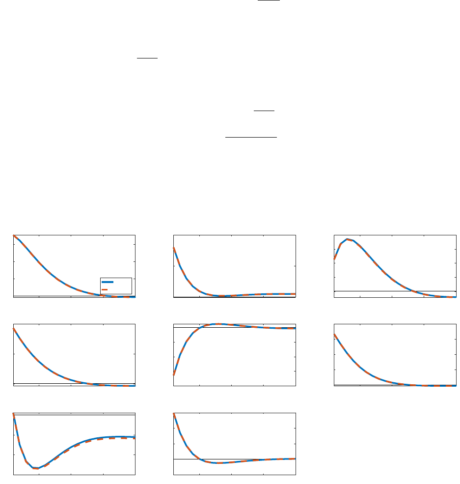
F RANK Household

In the representative agent model, the lifetime utility of the household is

∞

t=0

log C

− χ

1+η

1 + η

The ﬂow budget constraint is

t−1

+ mrs

(1 − τ)L

− C

− T

+ div

− X, (F.1)

The ﬁrst order conditions are

−1

= βR

−1

t+1

(F.2)

(1 − τ)mrs

χC

. (F.3)

G Conventional Monetary Policy

Figure G.1: Impulse responses under a monetary policy shock

5 10 15 20

0.2

0.4

0.6

output

RANK

HANK

5 10 15 20

0.5

consumption

5 10 15 20

0.5

1.5

investment

5 10 15 20

0.5

labor

5 10 15 20

-0.2

-0.15

-0.1

-0.05

policy rate

5 10 15 20

0.05

0.1

0.15

0.2

inflation

5 10 15 20

-0.3

-0.2

-0.1

deposit

5 10 15 20

-0.05

0.05

0.1

0.15

corp. bond spread

Notes: This ﬁgure plots the impulse responses of aggregate variables under a 0.25% monetary policy shock.

The blue solid lines are for the RANK model, and the red dashed lines are for the HANK model. X-axis is

time in quarters, and Y-axis is the percentage change from steady state.