Who gets jobs matters: monetary policy and the labour market in HANK and SAM

Working Paper Series

Who gets jobs matters: monetary

policy and the labour market in HANK

and SAM

Uroš Herman, Matija Lozej

Disclaimer: This paper should not be reported as representing the views of the European Central Bank

(ECB). The views expressed are those of the authors and do not necessarily reflect those of the ECB.

No 2850

Abstract

This paper ﬁrst provides empirical evidence that labour market outcomes for the less ed-

ucated, who also tend to be poorer, are substantially more volatile than labour market

outcomes for the well-educated, who tend to be richer. We estimate job ﬁnding rates and

separation rates by educational attainment for several European countries and ﬁnd that

job ﬁnding rates are smaller and separation rates larger at lower educational attainment

levels. At cyclical frequencies, ﬂuctuations of the job ﬁnding rate explain up to 80% of

the unemployment ﬂuctuations for the less educated. We then construct a stylised HANK

model augmented with search and matching and ex-ante heterogeneity in terms of ed-

ucational attainment. We show that monetary policy has stronger effects when the job

market for the less educated and hence poorer is more volatile. The reason is that these

workers have the most procyclical income coupled with the highest marginal propensity

to consume. An expansionary monetary policy shock that increases labour demand dis-

proportionally affects the labour market segment for the less educated, causing a strong

increase in their consumption. This further ampliﬁes labour demand and increases labour

income of the poor even more, amplifying the initial effect. The same mechanism carries

over to forward guidance.

JEL classiﬁcation: E40, E52, J64

Keywords: Heterogeneous agents, Search and matching, Monetary policy, Business cycles, Employ-

ment

ECB Working Paper Series No 2850

Non-technical summary

In this paper we ﬁrst provide a set of new empirical estimates of job ﬁnding and separation

rates by educational attainment, and their cyclical properties for several European countries.

We ﬁnd that job ﬁnding rates for the less educated (and more likely poor) workers are lower,

highly procyclical, and more volatile than for the better educated (more likely better well-

off) workers. We also ﬁnd that separation rates are higher, tend to be more volatile, and

often acyclical for the less educated workers. There are considerable differences across Eu-

ropean countries, with some countries where the labour market displays fewer differences

by educational attainment than in others. In all cases, ﬂuctuations in job ﬁnding rates seem

to contribute the most to ﬂuctuations in unemployment of the less educated at cyclical fre-

quencies, with the contribution of job ﬁnding rate ﬂuctuations exceeding 80% in countries

like Germany and France. We report similar evidence for the US. In all cases, the evidence

suggests that agents with low educational attainment face higher employment risk over the

business cycle than agents with high educational attainment.

We then build a stylised model with the search and matching framework embedded in

a HANK framework that attempts to capture these empirical properties. The model con-

siders the economy as composed of different labour market segments, where workers can

either stay in the same market segment and face its income risk, or exogenously switch to an-

other labour market segment, with different characteristics regarding wage ﬂuctuations and

(un)employment risk. These exogenous switches between labour market segments are rare

but persistent and can be thought of as persistent changes in the desirability for a particular

skill.

Labour market segments differ with respect to wage level, job ﬁnding probabilities, and

their cyclical properties. Each segment functions as a separate labour market with search

and matching frictions. This means that each labour market segment has an endogenous job

ﬁnding probability, which depends on ﬁrms’ incentives to create vacancies in that segment,

which in turn varies with economic conditions. Cyclical income ﬂuctuations for households

that stay in the same labour market segment occur because search frictions, combined with

wage rigidities, lead to an increased vacancy posting following an expansionary shock, which

increases job ﬁnding rates and therefore expected labour income within each labour market

segment. Because the intensity of vacancy posting differs across labour market segments,

the differences between labour market segments change over the business cycle and affect the

idiosyncratic labour income risk for households. In other words, the income loss/gain due to

exogenous shifts from one labour market segment to the other differs over the business cycle.

We use this framework to investigate the implications of such heterogeneous labour mar-

kets for monetary policy. We show that if poor workers obtain relatively more jobs after a

monetary expansion, which is consistent with empirical evidence for most countries we con-

sider, they also spend a larger proportion of the additional income, because their marginal

propensity to consume is higher. This ampliﬁes the aggregate demand increase, which leads

to more labour demand from ﬁrms that have to produce in order to meet consumption de-

ECB Working Paper Series No 2850

mand. Because the labour market for the poor is more sensitive to the business cycle, this

leads to a relatively stronger increase in employment of poorer households, which again leads

to a stronger increase in consumption. This works as an ampliﬁcation mechanism that makes

monetary policy more potent.

What turns out to be important for the ampliﬁcation is the asymmetry of the labour

market, in the sense that the labour market segment of the poor reacts more procyclically

than the labour market segments further to the right of the wealth distribution. We show that

this can be brought about by two mechanisms that amplify vacancy posting in the labour

market segment with lower educational attainment. One such mechanism is a relatively low

and hence more volatile ﬁrm surplus from hiring a worker from this labour market segment,

and the other is a higher wage rigidity in the segment. Either or both lead to more volatile

hiring for workers with lower educational attainment.

ECB Working Paper Series No 2850

1 Introduction

The distribution of wealth and the riskiness of income matter substantially for macroeco-

nomic ﬂuctuations in the standard heterogeneous agent New Keynesian (HANK) models

(Kaplan et al., 2018). An important issue in the literature has been the so-called earnings het-

erogeneity channel (Auclert, 2019), which has focussed on the incidence of a particular type

of earnings such as interest, dividends, labour income and taxation (Werning (2015), Broer

et al. (2018), and Hagedorn et al. (2018)). There was less emphasis on the incidence of labour

income itself over the business cycle for different households, even though labour income is

typically the most important source of income for the majority of households.

Labour literature tends to ﬁnd that workers face heterogeneous employment prospects

and, thus, income risk over the business cycle. For example, Elsby et al. (2010) document that

males, younger, less educated workers, and individuals from ethnic minorities experience

steeper rises in unemployment during all recessions. Similarly, Patterson (2023) ﬁnds that

earnings of individuals with higher marginal propensities to consume (i.e., young, black,

and poor) are more exposed to recessions.

Relatedly, Haltiwanger et al. (2018) document

that during the downturns, less educated and younger workers are more likely to exit to

nonemployment and less likely to get out of nonemployment. Hoynes et al. (2012) come

to a similar conclusion using individual-level Current Population Survey (CPS) and Merged

Outgoing Rotation Group (MORG) data.

Workers with such characteristics are more likely

to be poor. For example, in the Households Finance and Consumption Survey, the typical

ﬁnding is that younger and less educated households are more likely to be credit constrained

(see HFC (2016)).

Who is rich and who is poor matters in HANK models because households differ in

terms of their marginal propensities to consume. In this setting, it is important whether

household income (and income risk) is pro- or countercyclical because this matters for aggre-

gate demand, which in turn matters for general equilibrium effects on households’ incomes

(Werning (2015), Acharya and Dogra (2018), Bilbiie (2018)). Moreover, economic policies may

affect various segments of the wealth distribution differently, with the left tail typically being

more strongly affected (Amberg et al. (2022) and Broer et al. (2022)). Using administrative

data for the US, Guvenen et al. (2017) investigate how individual earnings vary across the

wealth distribution, and ﬁnd that the sensitivity of the workers to the business cycle, the

so-called “worker betas”, is higher at the bottom and at the top of the earnings distribution.

Kramer (2022) ﬁnds that the sensitivity is substantially higher at the bottom of the earnings

distribution (but not at the top) using German data. Moreover, he can attribute this to the

ﬂuctuations in the extensive margin rather than to wages. Auclert and Rognlie (2018) use

Mueller (2017) ﬁnds that during recessions, the pool of unemployed shifts towards high-wage workers.

Elsby et al. (2015) observe similar regularity, and they attribute it to compositional effect; during recessions,

the composition of the unemployment pool becomes skewed towards more attached individuals (i.e. male,

prime-aged, more educated) because they are less likely to exit the labour force.

Den Haan and Sedlacek (2014) develop a model where the least productive workers lose jobs ﬁrst during

the recession, and the most productive workers tend to get jobs ﬁrst during the boom.

ECB Working Paper Series No 2850

the results from Guvenen et al. (2017) to calibrate a function that rations labour of partic-

ular groups of households when wages are sticky, but the deeper underlying reasons why

and who gets/loses jobs in the boom/recession have been less thoroughly investigated. A re-

cent example of an approach that provides more micro-foundations for heterogeneous labour

market outcomes has been to use capital-skill complementarities (Dolado et al., 2021).

This paper ﬁrst provides new empirical evidence on job ﬁnding and separation rates by

educational attainment for several European countries, which is novel and of independent

interest. We ﬁnd that job ﬁnding rates for the less educated (and more likely poor) workers

are lower, highly procyclical, and more volatile than for the better educated (more likely

rich) workers. We also ﬁnd that separation rates are higher, tend to be more volatile, and

often acyclical for less educated workers. There are considerable differences across European

countries, with some countries where the labour market seems more homogeneous (with

fewer differences by educational attainment) than in others. In all cases, ﬂuctuations in job

ﬁnding rates contribute most to ﬂuctuations in unemployment of the less educated at cyclical

frequencies, with the contribution of job ﬁnding rate ﬂuctuations exceeding 80% in countries

like Germany and France. We report similar evidence for the US. In all cases, the evidence

suggests that agents with low educational attainment face higher employment risk over the

business cycle than agents with high educational attainment.

We then build a stylised model with the search and matching framework embedded in

a HANK framework that attempts to capture the above empirical regularities. The model

considers the economy as composed of different labour market segments, where workers can

either stay in the same market segment and face its income risk, or exogenously switch to

another labour market segment, with different characteristics regarding wage ﬂuctuations

and (un)employment risk. These exogenous switches between labour market segments are

rare but persistent and can be thought of as persistent changes in desirability for a particular

skill.

Labour market segments differ with respect to wage level, job ﬁnding probabilities,

and their cyclical properties. Each segment functions as a separate labour market with search

and matching frictions. This means that each labour market segment has an endogenous job

ﬁnding probability, which depends on ﬁrms’ incentives to create vacancies in that segment,

which in turn varies with economic conditions. Cyclical income ﬂuctuations for households

that stay in the same labour market segment occur because search frictions, combined with

wage rigidities, lead to an increased vacancy posting following an expansionary shock, which

increases job ﬁnding rates and therefore expected labour income within each labour market

segment. Because the intensity of vacancy posting differs across labour market segments,

the differences between labour market segments change over the business cycle and affect

the idiosyncratic labour income risk for households (the income loss/gain due to exogenous

shifts from one labour market segment to the other).

For instance, one can think of one incidence of such a switch looking at the data from a major job ﬁnding

intermediary, Indeed (Adrjan (2019)). These indicate that upon the announcement that the plant of British Steel

was scheduled to close, workers from that plant searched for jobs that were below their qualiﬁcation level. That

is, they searched for a job in what is effectively a different labour market segment.

ECB Working Paper Series No 2850

We use this framework to investigate the implications of such heterogeneous labour

markets for monetary policy. We show that if poor workers obtain jobs after a monetary

expansion (which is consistent with empirical evidence), they spend a larger proportion of

the additional income, because their marginal propensity to consume is higher. This ampliﬁes

aggregate demand, which leads to more labour demand from ﬁrms that have to produce

in order to meet consumption demand. Because the labour market for the poor is more

sensitive to the business cycle, this leads to a relatively stronger increase in employment of

poorer households, which again leads to a stronger increase in consumption. This works as

an ampliﬁcation mechanism that makes monetary policy more potent. What turns out to be

important for the ampliﬁcation is the asymmetry of the labour market, in the sense that the

labour market segment of the poor reacts more procyclically than the labour market segments

further to the right of the wealth distribution. We show that this can be brought about by

two mechanisms that amplify vacancy posting in the labour market segment with lower

educational attainment. One such mechanism is a relatively low and hence more volatile

ﬁrm surplus from hiring a worker from this labour market segment, and the other is a higher

wage rigidity in the segment. Either or both lead to more volatile hiring for workers with

lower educational attainment.

Our paper is most closely related to papers analysing economic ﬂuctuations in het-

erogeneous agents models with labour market frictions (see, for example, Den Haan et al.

(2017), Ravn and Sterk (2017)). However, our paper differs from the others in focusing on the

differences between labour market segments and their implications for shock transmission.

Compared to Ravn and Sterk (2016) and Ravn and Sterk (2017), we consider the interplay

between several labour market segments and allow agents to save. Den Haan et al. (2017)

allow agents to save in two assets and solve the model fully globally, but they analyse a

uniﬁed labour market. Gornemann et al. (2016) do not differentiate between the structure of

labour market segments and focus mostly on systematic monetary policy and the distribution

of incomes from assets and labour, while our focus is on labour market segments. Kramer

(2022) models the transition between labour market segments as endogenous using directed

search, while our setting, where educational attainment is predetermined, considers switches

between labour markets that require different levels of educational attainment as exogenous

(and slow relative to the business cycle frequency). Differently from Dolado et al. (2021), our

model generates different labour market outcomes by only relying on labour market search

frictions without the need for capital-skill complementarity.

The remainder of the paper is structured as follows. Section 2 presents the empirical

evidence on who obtains jobs and when. Section 3 describes the model, Section 4 discusses

the results, and Section 5 concludes.

ECB Working Paper Series No 2850

2 Who gets and who loses jobs

Employment outcomes of the well and less educated workers can differ markedly over the

business cycle. Education level can also serve as a proxy for income and wealth, and the

literature has shown that economic policies may affect households at a different point in the

wealth distribution differently (see, for example, Amberg et al. (2022) or Broer et al. (2022)).

This section provides novel empirical evidence for several European countries and the US

on who gets and who loses jobs at business cycle frequencies across educational attainment

levels, and what are the main driving forces behind it.

Before looking into the driving forces of unemployment ﬂuctuations, it is instructive

to examine the variability of unemployment rates across educational attainment levels for

selected European countries. Table 1 shows that the unemployment rate at the lowest educa-

tional attainment level is much more volatile than the aggregate unemployment rate and the

unemployment rates at higher education levels for all countries considered, indicating that

those with lower educational attainment are much more exposed to business cycle ﬂuctua-

tions. The remainder of this section examines the underlying forces that drive ﬂuctuations

in unemployment rates, focussing on job ﬁnding and separation rates and their behaviour at

business cycle frequencies.

Table 1: Variability of unemployment rates over business cycles

Volatility Relative volatility

σ(u

) σ(u

)/σ(u)

Country Sample Agg. L M H L M H

France 2003Q1-2019Q4 0.35 0.57 0.36 0.28 1.60 1.00 0.80

Germany 2005Q1-2019Q4 0.25 0.36 0.28 0.16 1.41 1.11 0.64

Greece 1998Q1-2019Q4 1.39 1.55 1.60 1.00 1.12 1.15 0.72

Italy 2001Q1-2019Q4 0.47 0.61 0.43 0.35 1.31 0.92 0.75

Spain 1998Q1-2019Q4 1.23 1.57 1.23 0.85 1.27 0.99 0.69

UK 2000Q1-2019Q4 0.37 0.61 0.41 0.25 1.65 1.11 0.66

Notes: The table reports standard deviations of cyclical components of unemployment rates u

, and relative

volatilities with respect to the aggregate unemployment rate u , by educational attainment. Agg. = aggregate,

L = Less than primary, primary, and lower secondary education, M = Upper secondary and post-secondary

non-tertiary education, and H = Tertiary education. We end the sample in Q4 2019 to exclude the COVID-19

period.

2.1 Job ﬁnding rates and separation rates by educational attainment in

Europe

To estimate job ﬁnding rates by educational attainment, we use data on unemployment spell

duration by educational attainment, available in European Union Labour Force Survey (EU–

LFS). In general, we follow the method by Shimer (2012), and its extension by Elsby et al.

(2013). The difference compared to Elsby et al. (2013) is that we have quarterly data on the

ECB Working Paper Series No 2850

duration of unemployment, so we can more directly relate outﬂows from unemployment to

Shimer’s approach (which is based on monthly data).

Using the approach in Shimer (2012), the monthly change in unemployment can be

written as follows

t+1

− u

= u

t+1

− F

, (1)

where u

is unemployment at monthly frequency, u

t+1

is the stock of unemployed with un-

employment duration of less than one month, and F

is the ﬂow out of unemployment.

Rearranging and solving for outﬂow probability F

, one obtains:

= 1 −

t+1

− u

t+1

, (2)

which can be used to get the (monthly) outﬂow hazard rate f

= −ln

(

1 − F

)

. (3)

Following Shimer (2012), we refer to f

as the job ﬁnding rate and to F

as the correspond-

ing job ﬁnding probability. The computation of this rate requires monthly data. However, as

pointed out by Elsby et al. (2013), one can use data at lower frequencies, and this may be more

convenient in labour markets that are less ﬂuid than the US labour market, as is typically the

case in Continental Europe. In particular, one can compute

= 1 −

t+d

− u

t+d

, (4)

where d is the number of months, and compute the (monthly) outﬂow hazard rate as

= −ln



1 − F



/d. (5)

We follow this approach, using quarterly data on unemployment by educational at-

tainment collected by Eurostat, and EU–LFS data on unemployment duration spells, also by

educational attainment.

We do so for d ∈ {3, 6, 12}, and for three levels of educational attain-

ment: (L) Less than primary, primary, and lower secondary education, (M) Upper secondary

and post-secondary non-tertiary, and (H) Tertiary education. We focus on large countries in

Europe. The reason for this is twofold. First, we have relatively few observations for shorter

unemployment spells due to the relatively less ﬂuid labour markets in Continental Europe,

as pointed out by Elsby et al. (2013). Second, the data is quarterly, and we distinguish by edu-

As pointed out by Elsby et al. (2013), there could be an issue of duration dependence for data at a lower

frequency, if the labour market is very ﬂuid, so that job ﬁnding rates and separation rates are high. However,

they note that this is less of a problem for most Continental European countries, where labour markets tend to

be less vibrant than in the US, and for which Elsby et al. (2013) ﬁnd no evidence for duration dependence.

Data are seasonal, so we ﬁrst compute 4-quarter moving averages to remove seasonal ﬂuctuations. The

advantage of this over seasonal adjustment of each series is that it preserves additivity, i.e., moving averages of

unemployed by educational attainment add up to the moving average of total unemployed; moving averages of

the employed and unemployed sum to the moving average of the total labour force.

ECB Working Paper Series No 2850

cational attainment, which further reduces the sample. This means that for smaller countries

with a relatively small sample of the Labour Force Survey, we have only a few observations,

especially in the group with the highest educational attainment. We focus on d = 3 in the

main text but also report additional estimates for d = 6 and d = 12.

Table 2: Monthly job ﬁnding rates

<12

Country Sample L

M H L M H L M H

France 2003Q1-2019Q4 0.043 0.059

0.068 0.044 0.059 0.067 0.042 0.055 0.061

Germany 2005Q1-2019Q4 0.055 0.064 0.063 0.055 0.063 0.064 0.049 0.054 0.057

Greece 1998Q1-2019Q4 0.032 0.026 0.031 0.040 0.033 0.035 0.039 0.035 0.036

Italy 2001Q1-2019Q4 0.054 0.063 0.077 0.054 0.063 0.073 0.045 0.052 0.058

Spain 1998Q1-2019Q4 0.081 0.081 0.089 0.080 0.080 0.087 0.068 0.069 0.075

UK 2000Q1-2019Q4 0.049 0.068 0.077 0.052 0.070 0.079 0.047 0.061 0.066

Notes: The table reports monthly job ﬁnding rates f

using (5). L = Less than primary, primary, and lower

secondary education, M = Upper secondary and post-secondary non-tertiary education, and H = Tertiary edu-

cation. Values are sample averages. We end the sample in Q4 2019 to exclude the COVID-19 period.

Table 2 reports monthly job ﬁnding rates based on our estimates that can be compared

to those in Elsby et al. (2013).

Three main results stand out in these estimates. First, there

are considerable differences across countries, with job ﬁnding rates ranging from less then

0.03 in Greece to above 0.08 in Spain. Second, the job ﬁnding rate rises with educational

attainment and is the highest for those with tertiary education and above (H). However, there

are exceptions, such as Greece and Spain, where the job ﬁnding rate does not increase (or

only mildly increases) with the level of educational attainment.

Finally, and consistently

with Elsby et al. (2013), we ﬁnd that duration dependence does not seem to play a role - our

estimates of levels and volatilities are similar for various durations.

With the estimates of job ﬁnding rates f

, it is possible to back out the corresponding

separation rates s

(and the corresponding separation probability S

). Shimer (2012) advocates

using the following formula, which accounts for the fact that a worker who loses a job can

ﬁnd a new one within the same period:

t+1



1 − e

−

(

)



+ s

+ e

−

(

)

, (6)

where l

is labour force and e

is employment (and l

= e

+ u

This equation allows

us to solve for the separation rate implicitly. We apply it to each educational attainment

Table 12 in appendix reports quarterly job ﬁnding probabilities F

that we use in Section 3 to calibrate the

model.

This may be due to public-sector employment reductions during the sovereign debt crisis, which might

have affected relatively more educated workers in the public sector, although we cannot verify this based on

our data.

Accounting for the possibility that workers can lose and ﬁnd a job within the period could in principle be

important in our case because of the quarterly data frequency. However, because we ﬁnd for all countries in our

sample that hazard rates f

and s

are low (as in Elsby et al. (2013)), this is less of a concern.

ECB Working Paper Series No 2850

level, using our estimates of job ﬁnding rates by educational attainment and by duration of

unemployment. The results are reported in Table 3.

Table 3: Monthly separation rates

<12

Country Sample L

M H L M H L M H

France 2003Q1-2019Q4 0.007 0.006

0.004 0.007 0.006 0.004 0.007 0.005 0.004

Germany 2005Q1-2019Q4 0.007 0.003 0.002 0.007 0.003 0.002 0.006 0.003 0.001

Greece 1998Q1-2019Q4 0.005 0.006 0.004 0.006 0.007 0.005 0.006 0.007 0.005

Italy 2001Q1-2019Q4 0.007 0.006 0.005 0.007 0.006 0.005 0.006 0.005 0.004

Spain 1998Q1-2019Q4 0.020 0.014 0.010 0.020 0.014 0.010 0.018 0.012 0.008

UK 2000Q1-2019Q4 0.005 0.004 0.003 0.005 0.004 0.003 0.005 0.004 0.002

Notes: The table reports monthly separation rates s

using (6). L = Less than primary, primary, and lower

secondary education, M = Upper secondary and post-secondary non-tertiary education, and H = Tertiary edu-

cation. Values are sample averages. We end the sample in Q4 2019 to exclude the COVID-19 period.

Separation rates in Table 3 are higher for lower educational attainments than for higher

educational attainment levels, except in Greece, where the separation rates are relatively

close for all three educational attainment groups. Overall, the evidence from job ﬁnding and

separation rates is consistent with the notion that the risk of becoming unemployed, and

not ﬁnding a job quickly once unemployed, is higher for workers with lower educational

attainment.

2.1.1 Cyclical properties of job ﬁnding and separation rates

Further characteristics that are of interest are the volatility and cyclical behaviour of the

estimated job ﬁnding and separation rates.

Table 4 reports the standard deviation and correlation of the cyclical components of the

estimated job ﬁnding rates with the cyclical component of the total unemployment rate.

Three characteristics stand out. First, the job ﬁnding rates of the least educated (L) tend

to be more volatile in some countries (France, Germany, the UK) than job ﬁnding rates of

those with better education, especially when considering unemployment for each particular

educational attainment level (note that the highest education level, H, is quite volatile mainly

because of very small samples for this segment, so the results should be interpreted with cau-

tion).

Second, job ﬁnding rates at all educational levels are procyclical (they are negatively

correlated with unemployment). Third, there is considerable heterogeneity across countries

regarding the cyclical properties across educational attainment levels. In Germany, the M and

In Appendix A.1, we also plot monthly job ﬁnding f

and separation rates s

by educational attainment

across selected European countries for different unemployment duration spells.

Cyclical components were obtained using the Hodrick-Prescott ﬁlter with the smoothing coefﬁcient of 1600,

applied to average monthly rates in the quarter, as in Fujita and Ramey (2009).

While we do not emphasise this aspect here, job ﬁnding rates for the least educated tend to also be highly

seasonal, especially in countries of Southern Europe. This is another indication that this segment of the labour

market features more risky jobs than the other segments.

ECB Working Paper Series No 2850

H educational levels are almost acyclical; in Italy, L is mildly procyclical, and M and H are

more procyclical than L. Similarly, procyclicality tends to increase mildly with educational at-

tainment in Spain, while in Greece, all educational levels are similarly procyclical. In France,

Germany, and the UK, lower educational attainment levels tend to be more procyclical.

Table 4: Cyclical properties of job ﬁnding rates

Rel.

own v

ol. Rel. aggregate vol. Corr. with agg.

σ( f

)/σ(U

) σ( f

)/σ(U) unemployment

Countr

y Sample L

M H L M H L M H

France

2003Q1-2019Q4 13.93 11.38

14.19 14.96 11.80 19.01 -0.61 -0.43 -0.56

Germany 2005Q1-2019Q4 16.51 12.58 16.03 15.86 13.99 22.98 -0.46 -0.19 -0.08

Greece 1998Q1-2019Q4 8.08 5.92 9.15 7.75 6.37 9.69 -0.39 -0.42 -0.41

Italy 2001Q1-2019Q4 11.38 12.12 16.67 11.83 12.04 19.17 -0.23 -0.41 -0.50

Spain 1998Q1-2019Q4 8.52 10.46 10.84 9.08 9.84 10.84 -0.59 -0.71 -0.80

UK 2000Q1-2019Q4 12.76 12.28 11.21 11.36 13.78 15.40 -0.34 -0.42 -0.26

Notes: The table reports standard deviations of cyclical components of monthly job ﬁnding rates relative to the

standard deviation of the cyclical component of each group’s unemployment U

, aggregate unemployment U,

and correlations of cyclical components of monthly job ﬁnding rates with the cyclical component of aggregate

unemployment, all based on d = 3 estimates. L = Less than primary, primary, and lower secondary education,

M = Upper secondary and post-secondary non-tertiary education, and H = Tertiary education. We end the

sample in Q4 2019 to exclude the COVID-19 period.

The same set of cyclical statistics as for the job ﬁnding rates is reported in Table 5 for

separation rates. Several results stand out. First, separation rates are less volatile than job

ﬁnding rates relative to all unemployment measures. Second, separation rates for the lowest

educational attainments tend to be much more volatile than those for higher educational

attainment levels. Third, in particular for Germany and France and to a lesser degree for the

UK, separation rates at the lower educational attainment levels are acyclical.

2.1.2 Contributions of job ﬁnding and separation rates to unemployment ﬂuctuations

An important question is which rate, the job ﬁnding rate or the separation rate, contributes

more to the unemployment rate ﬂuctuations over the business cycle. Following Fujita and

Ramey (2009), we decompose unemployment variability into contributions from the job ﬁnd-

ing and separation rates.

Speciﬁcally, Shimer (2012) shows that if the job ﬁnding and separa-

tion rates are constant during a period t, then the corresponding equilibrium unemployment

rate can be computed using job ﬁnding and separation rates as u

= s

/(s

+ f

). If trend

components are denoted by a bar, then the deviations of unemployment from the trend can

be written as





= (1 − u

)ln





− (1 − u

)ln

+ ε

, (7)

The implicit assumption is that the educational attainment of workers does not change materially at business

cycle frequencies.

ECB Working Paper Series No 2850

Table 5: Cyclical properties of separation rates

Rel. own vol. Rel. aggregate vol. Corr. with agg.

σ(s

)/σ(U

) σ(s

)/σ(U) unemployment

Country Sample L M H L M H L M H

France 2003Q1-2019Q4 1.02 0.83 0.29 1.10 0.86 0.39 -0.08 0.06 0.26

Germany 2005Q1-2019Q4 1.47 0.74 0.32 1.41 0.83 0.46 0.01 0.65 0.52

Greece 1998Q1-2019Q4 0.71 0.91 0.58 0.68 0.98 0.52 0.41 0.34 0.21

Italy 2001Q1-2019Q4 0.65 0.51 0.44 0.67 0.51 0.51 0.66 0.69 0.44

Spain 1998Q1-2019Q4 1.27 0.93 0.50 1.36 0.87 0.50 0.82 0.81 0.81

UK 2000Q1-2019Q4 0.81 0.50 0.28 0.72 0.56 0.38 0.23 0.47 0.66

Notes: The table reports standard deviations of cyclical components of monthly separation rates relative to the

standard deviation of the cyclical component of each group’s unemployment U

, aggregate unemployment U,

and correlations of cyclical components of monthly separation rates with the cyclical component of aggregate

unemployment, all based on d = 3 estimates. L = Less than primary, primary, and lower secondary education,

M = Upper secondary and post-secondary non-tertiary education, and H = Tertiary education. We end the

sample in Q4 2019 to exclude the COVID-19 period.

where ε

is the residual term. The above equation can be more compactly written as

= du

+ du

j f r

+ ε

, (8)

where du

and du

j f r

are the contributions of the separation rate and the job ﬁnding rate,

respectively. The variance of du

is then

Var(du

) = Cov(du

, du

) + Cov(du

, du

j f r

) + Cov(du

, ε

). (9)

This can be used to attribute the share of cyclical variation in unemployment rate that

is explained by the cyclical variations of the job ﬁnding rate β

j f r

, the cyclical variation of the

separation rate β

, and the cyclical variation of the residual β

j f r

Cov(du

, du

j f r

)

Var(du

)

, β

Cov(du

, du

)

Var(du

)

, and β

Cov(du

, ε

)

Var(du

)

. (10)

Table 6 reports the estimates of the contributions of the job ﬁnding rate and the separa-

tion rate to cyclical ﬂuctuations of unemployment rates (note that β

j f r

+ β

= 1). The

key ﬁnding is that in all countries, ﬂuctuations in the job ﬁnding rate are the main contributor

to cyclical ﬂuctuations in the unemployment rate. Moreover, this is overwhelmingly the case

for all countries at the lowest education level, where ﬂuctuations in the job ﬁnding rate typi-

cally explain more than half (and often more than 80%) of the ﬂuctuations in unemployment

rates, and more than the share explained by the cyclical ﬂuctuations of the separation rate.

These ﬁndings are broadly in line with the empirical evidence for Europe. Slacalek et al.

(2020) suggest that, based on unconditional estimates, the elasticities of employment responses

of hand-to-mouth households, and in particular of poor hand-to-mouth households, tend to

be large. While the estimates vary across countries, the sensitivity of employment of poor

ECB Working Paper Series No 2850

Table 6: Contributions to cyclical variation of unemployment

j f r

Country Sample L M H L M H

France 2003Q1-2019Q4 0.96 0.69 0.92 0.01 0.32 0.07

Germany 2005Q1-2019Q4 0.87 0.48 0.55 0.09 0.49 0.44

Greece 1998Q1-2019Q4 0.39 0.41 0.40 0.19 0.18 0.05

Italy 2001Q1-2019Q4 0.80 0.85 0.86 0.14 0.17 0.10

Spain 1998Q1-2019Q4 0.52 0.60 0.68 0.41 0.35¸ 0.28

UK 2000Q1-2019Q4 0.64 0.64 0.63 0.31 0.33 0.35

Notes: The table reports contributions of the ﬂuctuations of the job ﬁnding rate β

j fr

and of the separation rate

to cyclical ﬂuctuations of the unemployment rate. All is based on d = 3 estimates. L = Less than primary,

primary, and lower secondary education, M = Upper secondary and post-secondary non-tertiary education, and

H = Tertiary education. β

j fr

and β

do not add up to 1 due to the variance contribution of the residual.

hand-to-mouth households is at least 1.5-times larger than the aggregate employment. A sim-

ilar ﬁnding is reported by Dossche and Hartwig (2019), who look at “worker betas” across

the income distribution and ﬁnd signiﬁcantly higher worker betas in the lowest household

income quintile. This elasticity can be up to four times higher in the lowest quintile than

in the highest quintile. Kramer (2022) studies the procyclicality of earnings growth in Ger-

many and ﬁnds that the procyclicality is mostly driven by transitions from nonemployment

to employment (i.e. job ﬁnding rates), especially at the bottom of the income distribution.

Moreover, he ﬁnds that individuals at the bottom of the income distribution have lower job

ﬁnding rates than wealthy individuals and are more exposed to business cycle ﬂuctuations.

Both ﬁndings are in line with what we ﬁnd for Germany based on the aggregate data. Em-

pirical evidence conditional on a monetary policy shock (Lenza and Slacalek (2018) and Broer

et al. (2022)) also suggests that in Europe, incomes of poor households tend to react more

strongly to a monetary policy than the incomes of wealthier households.

2.2 Evidence from the US

For the US, compared to European countries, we have more detailed data along several di-

mensions. First, we have more granular data in terms of educational attainment level. Second,

data on new hires includes hires from inactivity. Finally, we also have some evidence that

wages at lower educational attainment are more rigid than wages at higher educational at-

tainment levels.

The latter will turn out to be important for the quantitative results in the

model.

We use publicly available Longitudinal Employer-Household Dynamics (LEHD) data

from the US Census Bureau. The LEHD database is constructed from various administra-

tive sources, such as Quarterly Census of Employment and Wages, Unemployment Insurance

earnings data, surveys and censuses. All the data we use are quarterly, seasonally adjusted

This is the main reason why we report the empirical evidence for the US in a separate subsection.

ECB Working Paper Series No 2850

and cover period between 2000Q2 and 2017Q3. If not otherwise stated, (net) hires and sepa-

rations are expressed as a share of employment.

Figures 1a and 1b plot hires from, and separations to, persistent nonemployment across

education groups. One can observe that the hiring rate and separation rate are inversely

related to educational attainment, i.e., less educated workers have larger inﬂow and outﬂow

rates to persistent nonemployment.

To get a clearer picture of who is more affected by business cycle ﬂuctuations, we look

at the difference between the two rates. Figure 2 shows net worker ﬂows—hires minus

separations—by educational attainment. It shows that during the recession, net hiring for

the group of workers with the lowest educational attainment declined much more than for

the group with the highest educational attainment; during downturns, the less educated

segments of the labour market experience more adverse developments than segments for the

more educated. This pattern is particularly notable during the Great Recession when the

net hiring for the group with less than high school dropped by more than twice as much as

for the group with the bachelor’s or higher degree. While less extreme, the same pattern is

observed during the milder 2001 recession.

Notably, at the onset of recovery, the net hiring in the groups with the lowest educational

attainment is also the one that exhibits the largest jump upwards. Again the pattern is such

that the upward jumps are more extreme for the less educated groups, and the magnitudes of

the increases decrease with education. This indicates that the groups with lower education,

while being those that are most exposed to the net job loss in the recession, are also the

groups who are the most exposed to net job gain when the recession is over.

Table 7 shows summary statistics for our sample. Less educated workers experience

larger inﬂow and outﬂow rates to nonemployment, and these rates are also more volatile.

This conﬁrms that less educated workers face a higher risk of going to, or coming from,

nonemployment. For example, the rate of hires and separations for the workers in the lowest

education group is two to three times larger than for the workers in the highest education

group, and the volatilities of these rates are about three times higher for the least educated

than for the most educated.

With the LEHD data, we, unfortunately, cannot calculate job ﬁnding rates, but only their

proxies across education groups. The reason is that a job ﬁnding rate is deﬁned as a ratio

of unemployed workers who ﬁnd a job over the number of unemployed. However, in the

LEHD data, we observe only hires from nonemployment, which is a broader concept than

unemployment, as it also includes workers who are not in the labour force. Nevertheless, we

report these ”rates” (expressed as a share of an average employment within the education

group) in the last row of Table 7, as they at least give some notion of the ranking of these

rates between education groups. Note that these proxies for job ﬁnding rates are increasing

with educational attainment (except for the group of less than high school, but this group is

very small in the data).

To further investigate whether workers with low(er) educational attainment face larger

ECB Working Paper Series No 2850

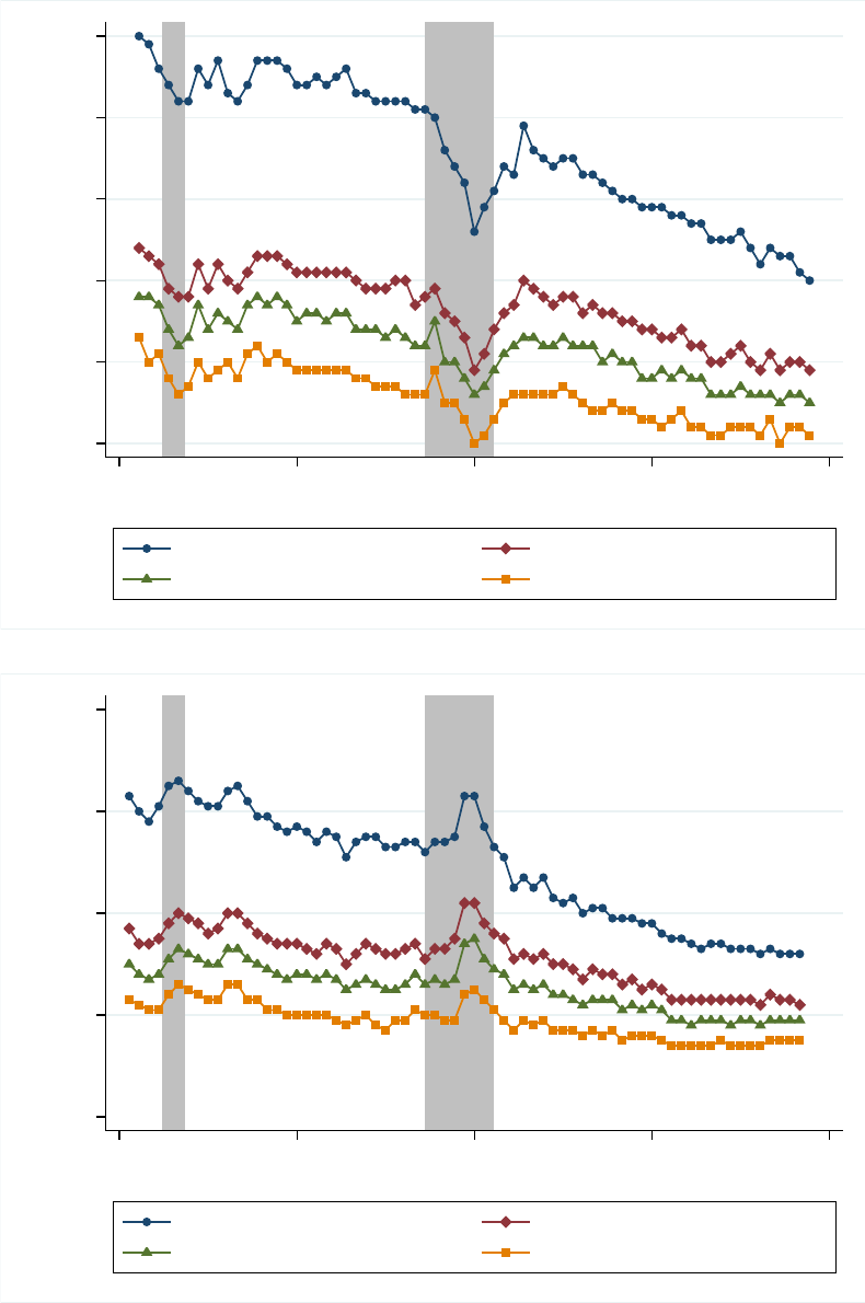
Figure 1: Hires and Separations to persistent nonemployment

(a) Hires

.03 .04 .05 .06 .07 .08

Hires from NonE

2000q1 2004q3 2009q1 2013q3 2018q1

date

Less than high school High school or equivalent, no college

Some college or Associate degree Bachelor’s or advanced degree

(b) Separations

.02 .04 .06 .08 .1

Separations to NonE

2000q1 2004q3 2009q1 2013q3 2018q1

date

Less than high school High school or equivalent, no college

Some college or Associate degree Bachelor’s or advanced degree

Notes: A worker is deﬁned as being a Hire from Persistent Nonemployment in quarter t, if she or he had no

main job in the beginning of the quarter t-1 and t, but had one at the end of quarter t. A worker is deﬁned as

undergoing a Separation to Persistent Nonemployment in quarter t, if she or he, had a main job in the beginning

of quarter t, and not at the end of quarter t or quarter t+1. Everything is expressed as a share of an average

employment within the education group. Shaded areas denote NBER recessions.

ECB Working Paper Series No 2850

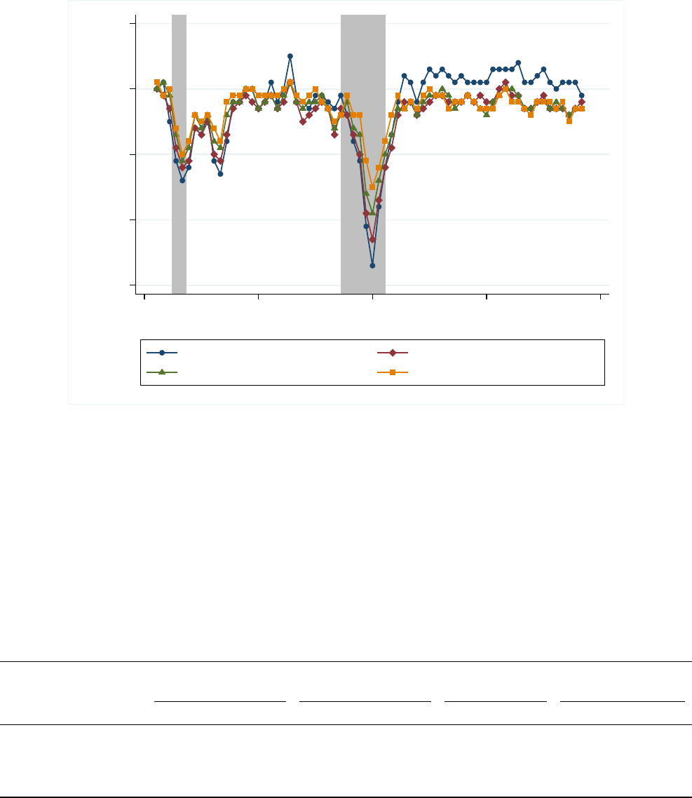
Figure 2: Net hires from persistent nonemployment

-.03 -.02 -.01 0 .01

Hires less Separations to NonE

2000q1 2004q3 2009q1 2013q3 2018q1

date

Less than high school High school or equivalent, no college

Some college or Associate degree Bachelor’s or advanced degree

Notes: Net hires is calculated as the difference between hires from and separations to persistent nonemploy-

ment, and it is expressed as a share of an average employment within the education group. Shaded areas denote

NBER recessions.

Table 7: Summary statistics

High

school or S

ome college or Bachelor’s degree or

Less than high school equivalent, no college Associate degree advanced degree

mean

sd mean sd

mean sd mean sd

Hir

es 0.066 0.0084 0.046

0.0043 0.041 0.0038 0.035 0.0032

Separations 0.069 0.011 0.051 0.0056 0.045 0.0045 0.038 0.0035

Hires less Separations -0.0025 0.0062 -0.0042 0.0045 -0.0035 0.0037 -0.0029 0.0030

Job ﬁnding rate proxy 0.782 0.218 0.614 0.187 0.714 0.294 0.776 0.350

Notes: (Net) hires and separations are rates and are expressed as a share of an average employment within the

education group.

ECB Working Paper Series No 2850

countercyclical employment risk, we estimate the following equation

i,t

= γ

+ β

educ

+ β

educ

× X

+ ϵ

i,t

, (11)

where Y

i,t

is either the (net) hire or separation rate, X

is the cyclical component of GDP,

educ

is workers’ educational attainment, γ

are time dummies to control for common shocks,

and ϵ

i,t

is the residual term. What we are interested in is the coefﬁcient on the interaction

term, which measures the differential responsiveness - across education groups - of net hiring

rate to a business cycle. Note that results have to be interpreted relative to the highest

education group.

Table 8: Worker ﬂows over the business cycle

(1)

(2) (3)

VARIABLES Net

hires Hires Separations

Less

than high school 0.000

0.030*** 0.030***

(0.000) (0.001) (0.001)

High school or equivalent, no college -0.001*** 0.011*** 0.012***

(0.000) (0.000) (0.000)

Some college or Associate degree -0.001** 0.006*** 0.007***

(0.000) (0.000) (0.000)

Less than high school × GDP cycle 0.123*** 0.079** -0.018

(0.036) (0.037) (0.056)

High school or equivalent, no college × GDP cycle 0.070*** 0.018 -0.044

(0.024) (0.019) (0.029)

Some college or Associate degree × GDP cycle 0.037 0.003 -0.031

(0.025) (0.020) (0.032)

ime FE X X

Observations 272 276 276

R-squared 0.9028 0.9713 0.9468

Robust

standard err

ors in parentheses

*** p<0.01, ** p<0.05, * p<0.1

Notes: (Net) hires, and separations are rates and are expressed as a share of an average employment within the

education group.

Table 8 reports the results from estimating Equation 11. Column 1 shows that the net hir-

ing rate of less educated workers is more sensitive to business cycles than the net hiring rate

of workers with the highest level of educational attainment. This implies that (countercycli-

cal) employment risk is the largest for the least educated workers, and it falls with increasing

educational attainment. Results are in line with Haltiwanger et al. (2018), who ﬁnd that

during recessions, workers with lower education are more likely to exit to nonemployment.

They also ﬁnd that conditional on ﬁrm productivity groups, hires and separations are more

cyclically sensitive for less educated workers. In columns 2 and 3, we separate the net hiring

We obtain it after applying the Hodrick-Prescott ﬁlter to a logarithm of seasonally adjusted real GDP. In

Appendix B.2, we also consider other business cycle measures, i.e. NBER recession episodes and the cyclical

component of the level of unemployment. The results do not materially change.

That is, relative to workers with a bachelor’s degree or an advanced degree.

ECB Working Paper Series No 2850

rate into hires and separations to see which margin is more important. We ﬁnd that only

hires are signiﬁcantly different across education levels; the hiring rate for the least educated

workers is more cyclically sensitive than for the workers with the highest education.

Appendix Table 18, we also estimate the sensitivity of changes in (net) hires and separation

rates to changes in GDP across education groups. Results conﬁrm our previous ﬁndings that

changes in (net) hiring rates of workers with lower education tend to be more sensitive to

changes in GDP, implying that they face larger employment and, therefore, income risk than

more educated workers.

2.2.1 Wage rigidity

For the US, we also have some evidence of differential wage rigidity across educational at-

tainment levels, which we lack for European countries.

Figure 3 plots the data from the matched Current Population Survey dataset (see Daly

et al. (2012)). The ﬁgure shows the percentage of workers who reported no change in their

wages over the past year by educational attainment. It shows that wages of less educated

workers tend to be stickier than wages of more educated workers. This regularity holds over

all business cycle phases and over a long time span.

While these data do not cover new

hires, they indicate that labour market segments by educational attainment have different

properties. More recent evidence of differential wage rigidity for new hires across education

levels is Doniger (2019), who ﬁnds (i) wages for new hires of least educated workers to

be acyclical, and that (ii) wage (pro)cyclicality increases with the educational attainment.

She also ﬁnds that after a monetary policy shock, less educated workers respond on the

employment margin while the more educated respond on the wage margin.

3 Model

To capture the characteristics of labour market segments described above and to investigate

their inﬂuence on the effectiveness of monetary policy, we build a small stylised model.

The core of the model is the heterogeneous agents New Keynesian model of McKay and

Reis (2016) and McKay et al. (2016), which we augment with search frictions on the labour

market. To account for the different labour market prospects faced by individual households,

we model each labour income level as its own labour market segment.

We assume that each labour market segment is populated by a continuum of households

and a continuum of labour ﬁrms. Labour ﬁrms post vacancies and households decide how

Interestingly, when we run regression on NBER recession episodes (see Table 16 in Appendix B.2), we ﬁnd

a statistically signiﬁcant difference in separation rates among education groups; low educated workers have

larger separation rates during downturn(s) relative to highly educated workers.

See Figure 31 in Appendix B.1 for the full sample.

In contrast, Haefke et al. (2013) and Kudlyak (2014) ﬁnd no evidence of nominal wage rigidity for new

hires, however as pointed out by Doniger (2019), they investigate a representative agent setting and do not

differentiate across educational attainment.

ECB Working Paper Series No 2850

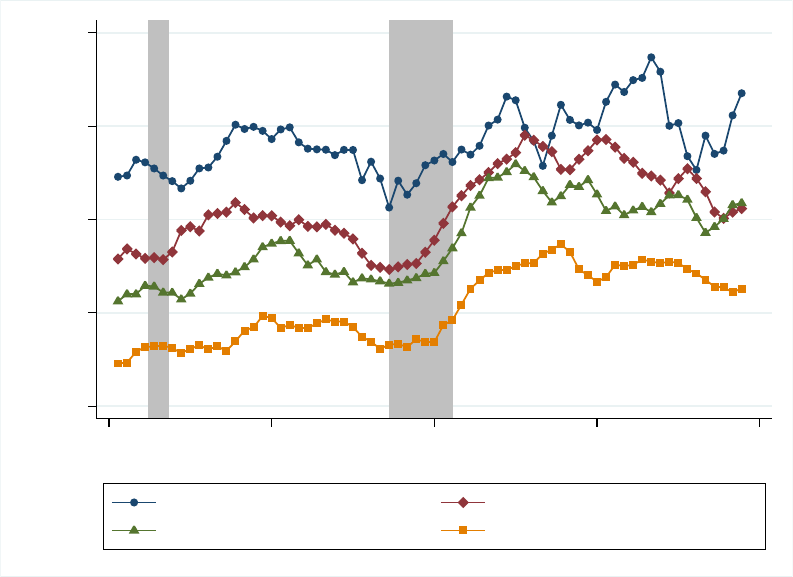
Figure 3: Wage rigidity by educational attainment

5 10 15 20 25

Nominal wage rigidity

2000q1 2004q3 2009q1 2013q3 2018q1

date

Less than high school High school or equivalent, no college

Some college or Associate degree Bachelor’s or advanced degree

Notes: Percentage of workers who saw no change in their wage over the past year by educational attainment.

Source: https://www.frbsf.org/economic-research/indicators-data/nominal-wage-rigidity/

many workers to send searching for jobs. Job search is subject to search frictions, and ﬁrms

and households take matching probabilities as given when deciding on how many vacancies

to post or how many workers to send to the market.

Markets are incomplete, and there is heterogeneity between households, but full insur-

ance within each household. Each household consists of a continuum of workers who have

the same level of labour productivity (educational attainment) and can be either employed or

unemployed. At the end of each period, workers bring their incomes home and the house-

hold as a whole decides on how much to consume and save, subject to prices and job ﬁnding

probabilities. This simpliﬁcation allows us that, within a household type, we can use the av-

erage rates of employment, unemployment, matching probabilities, and wages. In addition,

if there are no unemployment beneﬁts available, this assumption also prevents households

with no assets from having zero consumption. Note that this assumption still preserves the

cyclical risk of household income as a whole.

The household sends its workers to search for work at the beginning of each period.

They either ﬁnd work, in which case they bring home earnings, or they remain unemployed

and receive unemployment beneﬁts (if any). At the end of the period, all jobs terminate, and

the search starts again in the next period. This assumption allows us to avoid an additional

state variable (employment) for each labour market segment. Because we have three labour

market segments, this would add three additional endogenous state variables to the already

existing one endogenous continuous variable (asset holdings) and one exogenous (labour

ECB Working Paper Series No 2850

productivity process). Note that even in this case, the persistence of employment is implied

by the job ﬁnding probability in the labour market segment. That is, in segments with higher

job ﬁnding probabilities, employed workers are more likely to remain employed, even if they

separate every period, because they are more likely to ﬁnd a new job at the beginning of the

next period. That is, we can mimic income risk (and its ﬂuctuations) in each labour market

segment by the level and ﬂuctuations of the job ﬁnding probability.

The remainder of the model is similar to McKay et al. (2016). In the main text, we only

report the equations related to the search and matching frictions on the labour market in the

model, while the remaining equations are reported in Appendix C. The economy is populated

by a continuum of ex-ante identical households who face the following decision problem:

h,t

, z

h,t

) = max

h,t

h,t+1

h,t







1−γ

h,t

1 − γ

− η

1+η

h,t

1 + η

+ β

∑

h,t+1

(

h,t+1

h,t

)

t+1

h,t+1

, z

h,t+1

)







subject to

h,t

h,t+1

1 + r

= b

h,t

+ Bu

h,t

+ w

h,t

− τ

+ Π

, (12)

h,t

= l

h,t

+ u

h,t

, (13)

h,t

= p

h,t

, (14)

h,t

= (1 − p

h,t

, (15)

and

h,t+1

≥ 0. (16)

Here, c

h,t

is consumption of household with the educational attainment h at time t, b

h,t

are

its bond holdings at time t, r

is the real interest rate, s

h,t

is the number of searching workers

within household h at time t, l

h,t

is the number of employed workers within household h at

time t, u

h,t

is the number of unemployed workers within household h at time t, w

h,t

is the

real wage, and B are unemployment beneﬁts. τ

are taxes (levied as lump-sum depending

on the household’s labour endowment, and Π

are proﬁts from intermediate goods ﬁrms

and labour ﬁrms.

(

h,t+1

h,t

)

is the (exogenous) probability of transitioning between

labour market segments, and it follows a Markov process. The households take prices, taxes,

dividends, and unemployment beneﬁts as given.

We assume that all intermediate goods ﬁrms are held by an investment fund managed by

a risk-neutral manager, who collects proﬁts and distributes them as dividends to households

(households cannot trade in equities). Households are allowed to save by holding and trading

We assume that proﬁts from labour ﬁrms are given back to households as lump-sum but in proportion to

employment.

ECB Working Paper Series No 2850

riskless real bonds issued by the government. These bonds are in positive and constant net

supply, so households can partially self-insure by saving.

A household’s optimisation gives the following ﬁrst-order conditions with respect to the

choice variables

h,t

−γ

− λ

h,t

= 0, (17)

−

h,t

−γ

1 + r

+ β

∑

h,t+1

(

h,t+1

h,t

)

′

t+1

h,t+1

, z

h,t+1

) = 0, (18)

−η

h,t

+ p

h,t

− µ

h,t

+ (1 − p

h,t

)ξ

h,t

= 0, (19)

−q

h,t

+ µ

h,t

+ λ

h,t

= 0, (20)

−ξ

h,t

+ µ

h,t

+ λ

h,t

B = 0, (21)

where λ

h,t

is the multiplier on (12), µ

h,t

on (13), q

h,t

on (14), and ξ

h,t

on (15).

By eliminating the Lagrange multiplier on the budget constraint and applying the enve-

lope theorem, we get the standard Euler equation

h,t

−γ

= β(1 + r

)

∑

h,t+1

(

h,t+1

h,t

)

h,t+1

−γ

). (22)

3.1 Labour market

Labour market segments. There is a separate labour market for each productivity type

of households (in total, there are three labour market segments). On each labour market

segment, indexed by the productivity type z

, we have a separate matching function and

matching probabilities:

= ϕ

1−µ

, (23)

where m

is the number of matches in the market z

, ϕ

is the labour-market-segment-

speciﬁc matching efﬁciency, s

is the number of searching workers, and v

is the number

of vacancies. µ

is the elasticity of the matching function with respect to the number of

searching workers.

The matching probability for the worker, p

, is

= ϕ





1−µ

= ϕ

(

)

1−µ

, (24)

and the matching probability for the ﬁrm, p

, is

ECB Working Paper Series No 2850

= ϕ





−µ

= ϕ

(

)

−µ

. (25)

Households’ labour supply. Households send workers to search until the cost of searching

(measured in monetary terms) is equal to the expected earnings from searching. Rearranging

(17), (19), (20) and (21) delivers

h,t

+ u

h,t

)

−γ

h,t

= p

h,t

+ (1 − p

h,t

)B, (26)

where (l

h,t

+ u

h,t

) ≡ s

h,t

is the total amount of workers the household sends in the beginning

of the period to the labour market to search for jobs, c

−γ

h,t

is the marginal utility of consump-

tion, p

is a fraction of workers who ﬁnd a job and earn real wage w

, and (1 − p

) is a

fraction of workers who do not ﬁnd a job, but receive unemployment beneﬁts B. Condition

26 says that in equilibrium, the disutility of searching (measured in monetary terms) has to

be equal to the expected earnings from searching. The latter are weighted average of the ex-

pected real wage and unemployment beneﬁts, where the weight is the probability of getting

a job.

The setting of the model makes it clear where the sources of income ﬂuctuations come

from. The ﬁrst source, which is due to idiosyncratic labour productivity shocks that shift

households between labour market segments, is acyclical. These shocks can be thought of as

shocks that make a particular skill either more sought-after or less desired on the market.

This type of risk is fully taken into account by the households in our model. The second

type of income ﬂuctuation in our model is cyclical and comes from different labour market

conditions in labour market segments. These conditions depend on the state of the business

cycle and, in our model differ across the labour market segments. Because of these differ-

ences, transition from one labour market segment to the other implies a different gain or loss

of income, depending on the state of the business cycle.

Labour ﬁrms. We assume that each productivity segment of the labour market is populated

by a continuum of its own labour ﬁrms. Labour ﬁrms hire workers and sell their effective

labour as a homogeneous good at a competitive aggregate wage ω

to the intermediate-goods

ﬁrms. Each labour ﬁrm employs one worker. The value function of the labour ﬁrm is

= ω

h,t

− w

, (27)

where ω

h,t

is the total revenue received by the labour ﬁrm from selling labour services (one

worker provides labour services corresponding to his productivity z

h,t

, which is sold to the

Equation (26) also nests standard labour supply model; if p

= 1, so that everyone ﬁnds a job (implying

h,t

= 0), and B = 0, it reduces to the standard labour supply condition.

For example, automation in some industries have made workers with skills that can be automated less

sought-after, and workers who can program the machinery used for automation of these jobs more sought-after.

ECB Working Paper Series No 2850

intermediate-goods ﬁrm at the rate ω

). The labour ﬁrm pays the worker real wage w

and

returns proﬁts to the household as lump-sum.

The free-entry condition for labour ﬁrms is

= p

, (28)

where ψ

is the per-period vacancy posting cost in the labour market segment with produc-

tivity z

. In equilibrium, the labour ﬁrm’s optimality condition states that the per-period cost

of posting a vacancy is equal to the probability that the ﬁrm will ﬁnd a worker, times the

value of that worker for the ﬁrm, which is equal to the proﬁt the ﬁrm will earn in this period.

Wage determination. We consider two settings for wage determination. When wages are

fully ﬂexible, we assume that the wage rate that is paid to the workers in each segment is

a fraction (1 − α

) of the aggregate wage cost (which is the revenue received by the labour

ﬁrm),

= (1 − α

)ω

h,t

. (29)

The aggregate wage cost is determined in equilibrium as the cost that equates the labour

demand from intermediate goods ﬁrms with the labour services’ supply from labour ﬁrms.

When we analyse a setting with rigid wages, we follow Hall (2005) and model wage

rigidity as a weighted average of the wage that would be determined in the current period

(as described above), and a wage norm. For the wage norm we take the steady-state wage.

We allow wage rigidity to differ across labour market segments. The rigid wage is then

= [(1 − ω

)(1 − α

)ω

+ ω

(1 − α

)ω]z

h,t

, (30)

where ω

∈ [0, 1] is the weight of the wage norm in wage determination, and (1 − α

)ω is

the wage norm.

Relation to Nash bargaining. Here we show that our ﬂexible wage rule is just a particular

case of the standard Nash bargaining. With Nash bargaining, the wage is the outcome of

bargaining between workers and ﬁrms regarding the split of the total surplus generated by a

successful match. The solution to the Nash bargaining problem is

= (1 − χ

)(W

− W

), (31)

where χ

∈ (0, 1), is the bargaining power of the worker that can be labour-market-segment-

speciﬁc,

is the value of a job for a ﬁrm, and W

, W

are the value functions of being

employed and unemployed. The value functions for a ﬁrm and a worker are

This allows us to avoid introducing past wage as an additional state variable.

With χ

= 1, ﬁrms would have zero proﬁts (all the surplus goes to workers), but would still have to pay

positive vacancy posting costs which would prevent them from posting any vacancies.

ECB Working Paper Series No 2850

= ω

h,t

− w

, (32)

= w

− η

h,t

+ u

h,t

)

−γ

h,t

, (33)

= B − η

h,t

+ u

h,t

)

−γ

h,t

. (34)

To get the wage equation, one substitutes (32), (33), and (34) into (31) yielding

= χ

(ω

h,t

− B) + B, (35)

which means that the bargained wage a worker receives is equal to the outside option (in

our case unemployment beneﬁts) and a fraction (χ

) of the surplus from a successful match.

Note that the larger the χ

, i.e. the larger the bargaining power of the worker, less “sticky”

is the real wage. If we set B = 0, so that there are no unemployment beneﬁts, and deﬁne

≡ (1 − α

), we get exactly (29).

Finally, in order to see how the wage depends on the labour market developments, we

substitute (28) and (25), together with (33), and (34) into (31) to obtain

1 − χ



(θ

)



+ B, (36)

which states that the negotiated wage is increasing in bargaining power of the worker χ

vacancy posting cost (ψ

), labour market tightness θ

, and decreasing in matching efﬁciency

3.2 Calibration

The model is quite stylised and we largely rely on standard values from the literature to

calibrate it. However, for the labour market, we do match some of the properties reported in

the empirical section of the paper. In particular, we calibrate the model to match job ﬁnding

probabilities by educational attainment and their relative volatility. We also perform several

experiments illustrating how the model properties depend on the calibration choices.

The calibration of production and utility functions follows McKay et al. (2016), and is

reported in Table 9.

Idiosyncratic risk of transiting from one labour market segment to the other is calibrated

using the transition matrix from McKay et al. (2016) who use the persistent component of

wage process from Floden and Lind

e (2001), approximated using a 3-state Markov process

with the transition matrix P:

ECB Working Paper Series No 2850

Table 9: Utility function and production function

Parameter Value

Risk aversion γ 2

Frisch elasticity (inverse) η

Disutility weight for labour η

Markup µ 1.2

Price rigidity θ 0.15

P =







0.966 0.034 0

0.017 0.966 0.017

0 0.034 0.966







This matrix gives rise to the population shares [0.25 0.5 0.25], for each labour market

segment, ”poor”, ”middle”, and ”rich”. These transition probabilities do not vary over the

business cycle so that the mass of households in each segment is constant.

The calibration of the labour market is reported in Table 10. Labour endowment corre-

sponds to the level of wages in each labour market segment and follows McKay et al. (2016).

The differences in wage level also give rise to differences in the wealth distribution, which

reﬂects, to some extent, the differences in the wage level (hence the labels ”poor”, ”mid-

dle”, and ”rich”). The calibration of matching elasticities relies on the standard values from

Petrongolo and Pissarides (2001). Since wages in Continental Europe and in Germany are

fairly rigid, and since we do not have good data on the differences in the wage rigidity by

educational attainment levels, we assume that the degree of wage rigidity is equal across

all labour market segments.

We investigate the implications of this assumption when we

recalibrate the model to US data.

We use the calibration of the entrepreneur’s share and the vacancy posting cost to match

the job ﬁnding probability for the typical case where this probability increases by educational

attainment. We have picked the values that very closely correspond to the values found for

Germany. The model is quarterly, and we report quarterly probabilities corresponding to the

monthly rates from Section 2 in Table 12 in the appendix. Because the job ﬁnding probability

depends on the ratio of vacancy posting cost and the entrepreneur’s share, we could have

ﬁxed one and used the other to match the job ﬁnding probability. However, we wanted also

to match the relative volatility of the labour market segments, which in Germany are more

volatile and much more procyclical for the low-educated (see Table 14 in the appendix). To do

so, we follow the idea in Hagedorn and Manovskii (2008), who propose to solve the puzzle of

low volatility of labour market variables in the standard search-and-matching model (Shimer,

2005) by calibrating the entrepreneur’s share to be small. We set the entrepreneur’s share to

be smaller in the labour market segment with the lowest educational attainment, where we

Our choice of wage rigidity calibration implies that wages adjust only by half of what they would if they

were ﬂexible.

ECB Working Paper Series No 2850

observe higher labour market volatility, and then adjust the vacancy posting cost to match

the job ﬁnding probability.

Table 10: Matching function and labour ﬁrms

Parameter Poor Middle Rich

Labour endowment z

0.4923 1.0000 2.0313

Matching elasticity µ

0.5 0.5 0.5

Matching efﬁciency ϕ

0.6 0.6 0.6

Vacancy posting cost ψ

0.01 0.11 0.37

Entrepreneur’s share α

0.01 0.06 0.11

Wage rigidity ω

0.5 0.5 0.5

Job ﬁnding probability p

0.14 0.16 0.18

While modelled on Germany, this calibration is meant to represent the typical case found

in the labour data also for other European countries, such as France. We refer to this cali-

bration as ”Poor more volatile”. There are, however, countries such as Spain where there

seem to be fewer differences in terms of volatility and cyclicality between different labour

market segments (Table 14 in the appendix). To illustrate the difference this makes, we also

report simulations for the recalibrated model, where labour market segments are similar in

terms of their volatilities. We do this by matching job ﬁnding probabilities for Spain (0.20 for

each labour market segment) and by equalising entrepreneurs’ share across labour market

segments (at 0.05), which makes labour ﬁrms’ surplus and hence vacancy posting equally

cyclical for all segments of the labour market. We refer to this calibration as ”All equally

volatile”. Finally, as a counterfactual, we also simulate a calibration where we still keep the

volatility of the labour market outcomes of the less educated higher than that for the highly-

educated, but we make the difference less pronounced. We refer to this case as ”Poor less

volatile”.

4 Results

4.1 Calibration for European countries

We ﬁrst simulate a standard monetary policy shock, where the central bank temporarily

lowers the real interest rate by half a percentage point.

The results are reported in Figures

4 to 6.

We follow McKay et al. (2016) and assume that because prices are sticky, a central bank can directly control

the real interest rate in the short run. We use a persistence of 0.6 for the AR(1) process governing the shock.

ECB Working Paper Series No 2850

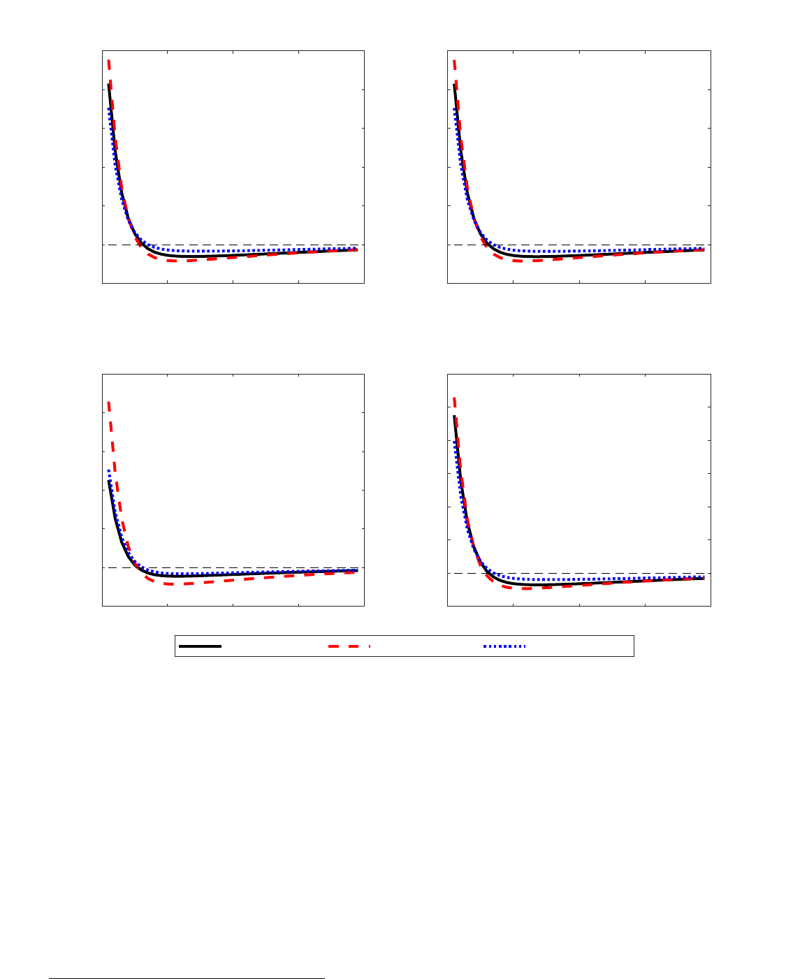
Figure 4: Effectiveness of monetary policy depending on who gets jobs

0 10 20 30 40

-0.1

0.1

0.2

0.3

0.4

0.5

Output (Consumption)

0 10 20 30 40

-0.1

0.1

0.2

0.3

0.4

0.5

Labour

0 10 20 30 40

-0.05

0.05

0.1

0.15

0.2

0.25

Dividends

0 10 20 30 40

-0.1

0.1

0.2

0.3

0.4

0.5

0.6

Total labour income (pre-tax)

Poor less volatile Poor more volatile All equally volatile

Notes: All variables are reported in percent deviations from the steady state. Units on the horizontal

axis are quarters.

Figure 4 reports results for the aggregates. The red dashed line represents our bench-

mark calibration in Table 10, where the labour market segment for the less educated house-

holds is calibrated to be more volatile than the other labour market segments, in line with

the data for Germany. For comparison, the full black line shows the case where the labour

market outcomes for the less educated are only half as volatile as the benchmark case (but

still more volatile than the other two labour market segments).

Everything else is kept the

same, which allows us to discuss the implications of labour market volatility for aggregate

ﬂuctuations. Finally, we also plot a case where the volatility of labour market outcomes is

For this speciﬁcation, entrepreneur’s shares α

in Table 10 now read [0.02, 0.06, 0.11].

ECB Working Paper Series No 2850

similar across all labour market segments, which would correspond to countries like Spain

(shown as a dotted blue line).

The key property to note is that aggregate ﬂuctuations tend to be ampliﬁed when the

labour market segment of the poor is more volatile. The initial output response is, for in-

stance, 17% higher for the red dashed line compared to the full black line, and this is similar

for aggregate labour and labour income responses. The difference in the magnitude of re-

sponses are even larger when compared to the symmetric case. Dividends are procyclical

due to sticky wages.

To understand the mechanism behind these results, it is instructive to look at the dis-

aggregated quantities. Figures 5 and 6 report impulse responses of the main variables of

interest by labour market segments. First, note in Figure 5 that labour of the poor households

increases substantially in the benchmark case with the labour market outcomes of the poor

more volatile, while labour of the rich households only increases on impact and then falls.

This becomes less pronounced if we make the labour market for the poor is less procyclical.

At the same time, consumption of the poor increases markedly in the benchmark case and

follows the pattern of the labour responses if we reduce the volatility in the labour market

segment for the poor. Consumption of the rich is almost unaffected, as they can smooth

their consumption by changing their asset holdings. Wages respond symmetrically across

all labour market segments, but with the different magnitude for each case considered, be-

cause they are determined by the aggregate labour demand and labour supply (recall that

the calibrated wage rigidity is the same in all cases shown).

Figure 6 provides an explanation for these observations. When the labour market of

the poor is more volatile, ﬁrms post relatively more vacancies in this labour market segment

during the expansion. This is because labour ﬁrm proﬁts in this segment are small, in line

with Hagedorn and Manovskii (2008), so they increase by more in percentage terms after a

positive shock whenever there is some wage rigidity. With more vacancies labour market

tightness in the segment increases, and with it also the job ﬁnding probability, causing more

employment and more labour income for the poor. Households in this labour market segment

have a high marginal propensity to consume, which is why their consumption increases

strongly. Despite the fact that this labour market segment is small and that consumption of

households in this segment is also small, the increase in consumption is sufﬁcient to increase

aggregate demand, which in turn leads to more labour demand and again more hiring from

the poor labour market segment, leading to further ampliﬁcation.

More employment in the poor labour market segment, in part, crowds-out employment

in the rich labour market segment, which is why we see a decline in labour in that segment

for the benchmark case. Note that this is not because ﬁrms would not want to hire from this

segment (tightness still increases) but because wages and the matching probability in this

In our model, all dividends are given as lump-sum to the rich households, who can smooth consumption,

so that cyclical properties of dividends do not play an important role. Note that because dividend income is also

procyclical, it matters less if we distribute it equally. This is in contrast to McKay et al. (2016), where households

that receive a substantial proportion of their income in the form of countercyclical dividends can even see their

total income fall after a monetary expansion.

ECB Working Paper Series No 2850

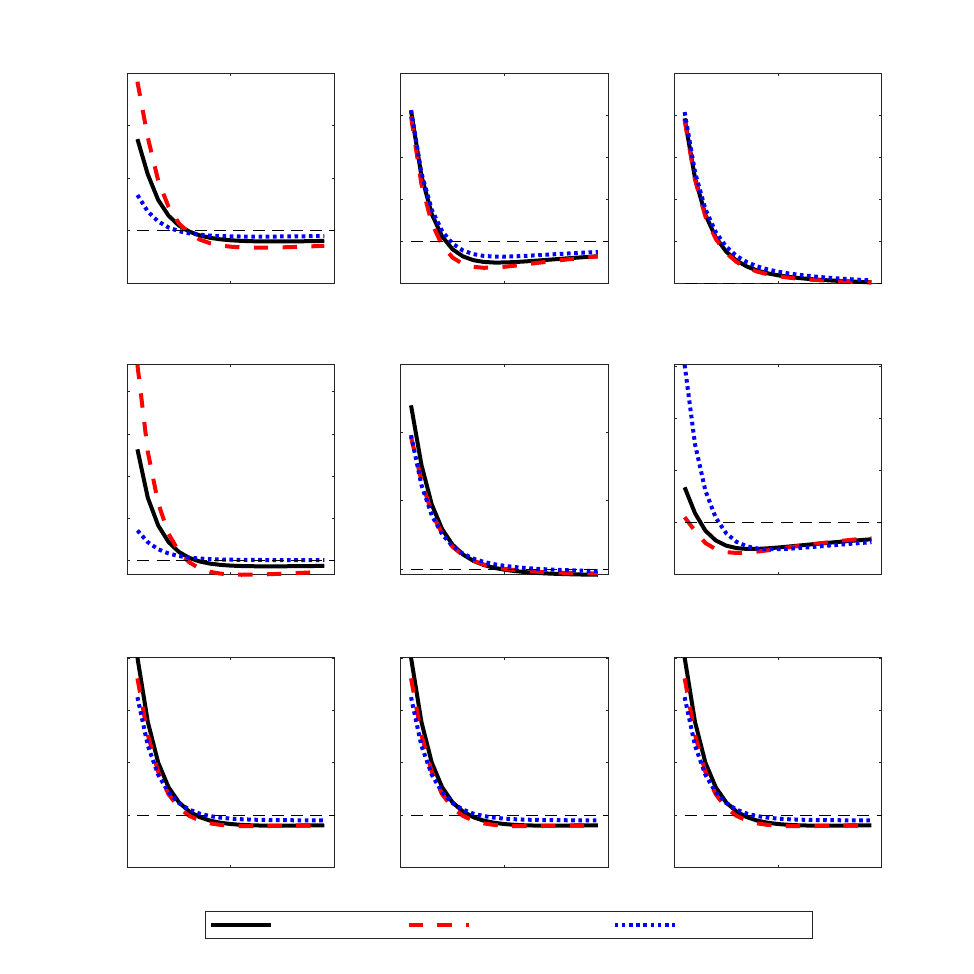
segment do not rise enough to induce the richer households to supply more labour. When

labour market segments are similar in terms of their cyclical behaviour, as is the case for

Spain-like calibration (dotted blue lines), there is little crowding-out on the labour market by

the poor households, which leads to a lower income and consumption response. The same

mechanisms apply to the transmission of forward guidance, reported in Appendix D.

Figure 5: Effectiveness of monetary policy by groups (1)

0 10 20

-0.5

0.5

1.5

Consumption

Poor

0 10 20

-0.1

0.1

0.2

0.3

0.4

Middle

0 10 20

0.1

0.2

0.3

0.4

0.5

Rich

0 10 20

0.5

1.5

Labour

0 10 20

0.2

0.4

0.6

0 10 20

-0.1

0.1

0.2

0.3

0 10 20

-0.01

0.01

0.02

0.03

Wages

0 10 20

-0.01

0.01

0.02

0.03

0 10 20

-0.01

0.01

0.02

0.03

Poor less volatile Poor more volatile All equally volatile

Notes: All variables are reported in percent deviations from the steady state. Units on the horizontal

axis are quarters.

ECB Working Paper Series No 2850

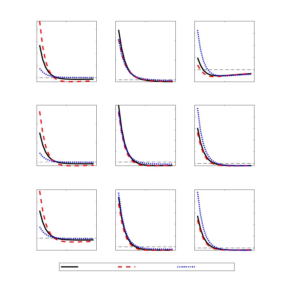
Figure 6: Effectiveness of monetary policy by groups (2)

0 10 20

0.5

1.5

Labour income

Poor

0 10 20

0.2

0.4

0.6

Middle

0 10 20

-0.1

0.1

0.2

0.3

0.4

Rich

0 10 20

Tightness

0 10 20

0.2

0.4

0.6

0.8

0 10 20

0.2

0.4

0.6

0.8

0 10 20

-0.1

0.1

0.2

0.3

0.4

Prob.-worker

0 10 20

0.02

0.04

0.06

0.08

0.1

0 10 20

0.02

0.04

0.06

0.08

0.1

Poor less volatile Poor more volatile All equally volatile

Notes: All variables are reported in percent deviations from the steady state, except probabilities,

which are in percentage points. Units on the horizontal axis are quarters.

4.1.1 The role of wage rigidity

The results shown above are, in addition to the friction due to market incompleteness, driven

by the interaction of two frictions, wage rigidities and search frictions. This subsection ex-

plains the role of wage rigidity in generating the ampliﬁcation after a monetary expansion.

To do so, we re-run the monetary policy shock in calibration to Germany, but this time with

fully ﬂexible wages. The aggregate results are reported in Figure 7, and the results for groups

by educational attainment in Figures 8 to 9. The red dashed line shows the benchmark results

reported above, while the dotted black line shows the case with fully ﬂexible wages.

ECB Working Paper Series No 2850

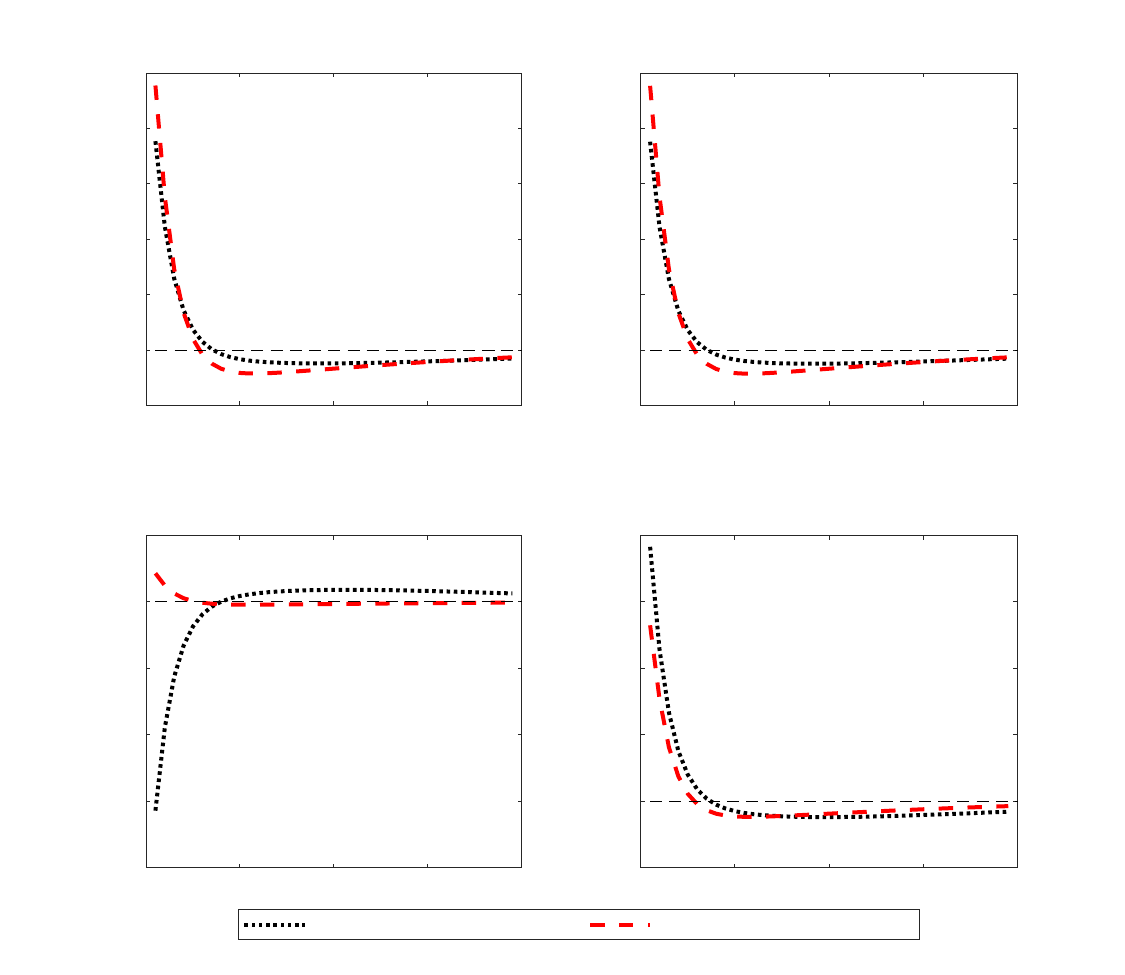
If we ﬁrst turn to Figure 7, we see that after a monetary expansion, the aggregate labour

income increases by more when wages are fully ﬂexible, but aggregate output and labour

increase by less, and dividends fall (note that the latter is a standard result in New Keynesian

models with sticky prices and ﬂexible wages).

Figure 7: The role of wage rigidity - aggregate

0 10 20 30 40

-0.1

0.1

0.2

0.3

0.4

0.5

Output (Consumption)

0 10 20 30 40

-0.1

0.1

0.2

0.3

0.4

0.5

Labour

0 10 20 30 40

-2

-1.5

-1

-0.5

0.5

Dividends

0 10 20 30 40

-0.2

0.2

0.4

0.6

0.8

Total labour income (pre-tax)

Poor more volatile, flexible wages Poor more volatile, sticky wages

Notes: All variables are reported in percent deviations from the steady state. Units on the horizontal

axis are quarters.

ECB Working Paper Series No 2850

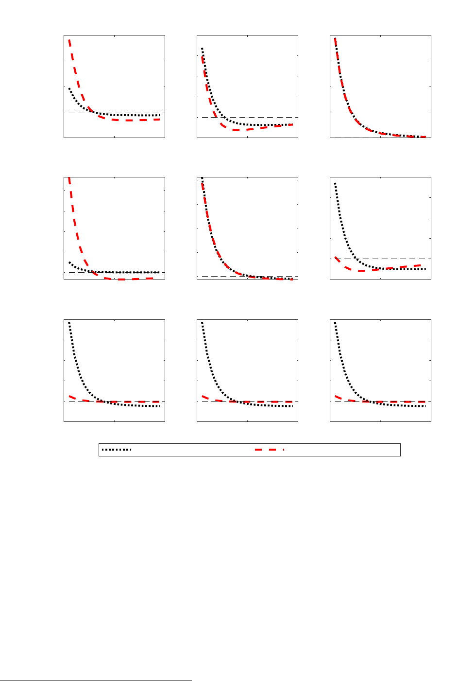
Figure 8: The role of wage rigidity by groups (1)

0 10 20

-0.5

0.5

1.5

Consumption

Poor

0 10 20

-0.1

0.1

0.2

0.3

0.4

Middle

0 10 20

0.1

0.2

0.3

0.4

Rich

0 10 20

0.5

1.5

Labour

0 10 20

0.1

0.2

0.3

0.4

0 10 20

-0.1

0.1

0.2

0.3

0.4

0 10 20

-0.1

0.1

0.2

0.3

0.4

Wages

0 10 20

-0.1

0.1

0.2

0.3

0.4

0 10 20

-0.1

0.1

0.2

0.3

0.4

Poor more volatile, flexible wages Poor more volatile, sticky wages

Notes: All variables are reported in percent deviations from the steady state. Units on the horizontal

axis are quarters.

The explanation for the result can be found by looking at Figures 8 and 9, where we see

that with ﬂexible wages, most of the difference in the labour response is concentrated in the

segments of poor and rich workers, with the poor working less in the case of ﬂexible wages

and the rich working more (both compared to the sticky wage case). Part of the reason is that

the rich households receive dividends, which fall in the case of ﬂexible wages, increasing the

labour supply of these households. A more important reason is that with ﬂexible wages, the

surplus of labour ﬁrms is less responsive for the poor compared to the benchmark case, and

given our calibration, it is also equally responsive across all labour market segments.

As a

Recall that this is because we calibrate vacancy posting costs in proportion to labour productivities of

ECB Working Paper Series No 2850

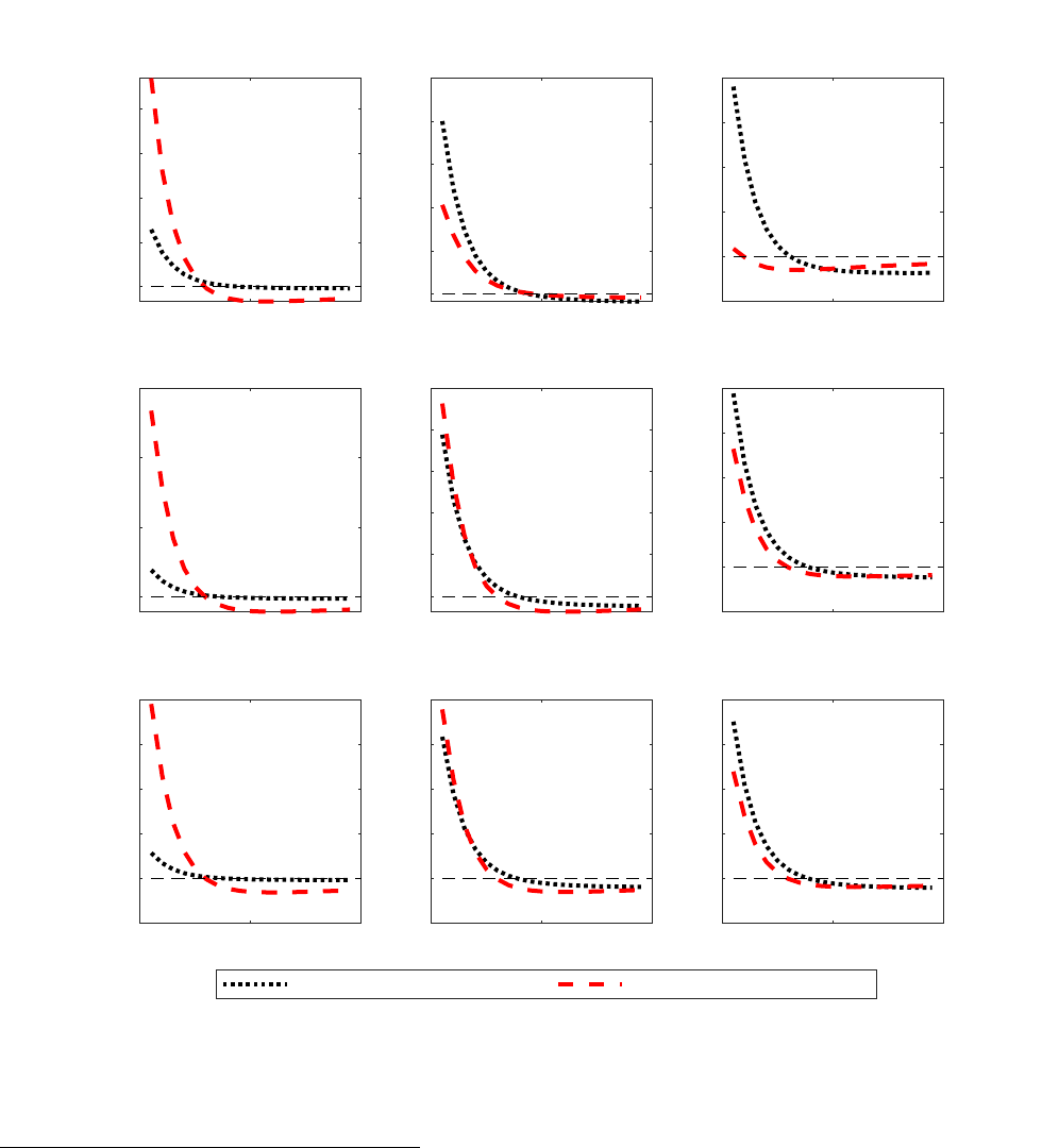
result, labour market tightness in Figure 9 increases approximately equally across all labour

market segments and is not disproportionally tilted towards the poor as in the benchmark

case. Compared to the sticky wage case, more jobs go towards the rich and middle-income

households, who have lower MPCs, so that the increase in aggregate demand, output, and

employment is lower. The ampliﬁcation effect due to disproportionate hiring in the poor

labour market segment is also not as strong as in the benchmark case. Dividends fall because

a higher wage increase is required to induce workers to supply more labour.

Figure 9: The role of wage rigidity by groups (2)

0 10 20

0.5

1.5

Labour income

Poor

0 10 20

0.2

0.4

0.6

0.8

Middle

0 10 20

-0.2

0.2

0.4

0.6

0.8

Rich

0 10 20

Tightness

0 10 20

0.2

0.4

0.6

0.8

0 10 20

-0.2

0.2

0.4

0.6

0.8

0 10 20

-0.1

0.1

0.2

0.3

0.4

Prob.-worker

0 10 20

-0.02

0.02

0.04

0.06

0.08

0 10 20

-0.02

0.02

0.04

0.06

0.08

Poor more volatile, flexible wages Poor more volatile, sticky wages

Notes: All variables are reported in percent deviations from the steady state, except probabilities,

which are in percentage points. Units on the horizontal axis are quarters.

households.

ECB Working Paper Series No 2850

4.2 Calibration for the US and differentials in wage rigidities

So far, we have always assumed that wage rigidity is the same for all labour market segments,

i.e., we have not relied on differences in wage rigidities across labour market segments. This

is because we have little hard evidence for European countries that some labour market seg-

ments have more rigid wages than the others, although this may be the case due to different

degrees of unionisation. However, we do have some evidence of differences in wage rigidity

in the US, and this section looks into the effects of such differences.

First, recall that the evidence for the US reported in Figure 3 that suggests that wages

are more sticky in the labour market for workers with low educational attainment. This is

important in our model because differences in wage rigidity affect the volatility of a labour

ﬁrm’s surplus and, therefore, vacancy posting. To investigate this issue, we recalibrate the

model again, this time to the US (see Table 11), and conduct the following experiments. First,

we consider fully ﬂexible wages across all labour market segments. Second, we make all

wages equally rigid. Third, we make rigid only wages of the labour market segment for the

poor.

Table 11: Matching function and labour ﬁrms, US calibration

Parameter Poor Middle Rich

Vacancy posting cost (fraction of lab. end.) ψ

0.06 0.05 0.04

Matching efﬁciency ϕ

0.6 0.6 0.6

Entrepreneur’s share α

0.02 0.05 0.10

Wage rigidity, ﬂexible ω

0 0 0

Wage rigidity, rigid poor ω

0.5 0 0

Wage rigidity, all rigid ω

0.5 0.5 0.5

Job ﬁnding probability p

0.60 0.70 0.80

We repeat the simulation of an expansionary and persistent monetary policy shock

across the three experiments. First, we consider the ﬂexible-wage case, which is shown in

Figures 10, 11 and 12 in full black lines. As one alternative, we assume wages are more rigid

in the labour market segment of the less educated (and therefore poorer) households. This

setup implies that in response to an expansionary monetary policy shock, labour ﬁrms post

more vacancies in lower-paying segments with more rigid wages because ﬁrm proﬁts in this

segment increase by more. Figure 10 shows the result of this experiment in dashed blue lines.

Finally, we consider the case where all groups have equally rigid wages, which is shown in

red dashed lines. Figures 11 and 12 show the effects by groups of households (each column

is one group of households by their labour productivity).

Our main result is that if wages of the poor are rigid, so that they obtain more jobs, then

output increases by more than it does when all wages are ﬂexible, and also more than in the

Because of high job ﬁnding probabilities in the US and because we use a Cobb-Douglas matching function,

it could happen that matching probability exceeds 1 if the shock is large. During the computation, we impose

the restriction that if this happens, the matching probability is set to 1.

ECB Working Paper Series No 2850

case where all wages are equally rigid. The difference is not negligible, given that the strength

of the output response on impact when wages of the poor are rigid is about 0.5%, compared

to about 0.4% in the ﬂexible-wage and the rigid-wage cases. This is even more so given that

the group of poor households is relatively small in the model (25% of the population).

Figure 10: Effectiveness of monetary policy depending on who gets jobs

0 10 20 30 40

-0.1

0.1

0.2

0.3

0.4

0.5

Output (Consumption)

0 10 20 30 40

-0.1

0.1

0.2

0.3

0.4

0.5

Labour

0 10 20 30 40

-1.5

-1

-0.5

Dividends

0 10 20 30 40

-0.2

0.2

0.4

0.6

0.8

Total labour income (pre-tax)

Poor less volatile Poor more volatile All equally volatile

Notes: All variables are reported in percent deviations from the steady state. Units on the horizontal

axis are quarters.

The mechanism that gives rise to this result is similar to the ones discussed above for

European countries, just that here the strong increase in labour ﬁrm surplus in the poor

labour market segment is ampliﬁed by the interaction both lower entrepreneur’s share and

higher wage stickiness in the labour market segment for the poor (dashed blue lines). Note

that this result is not obvious, because more rigid wages for the poor also mean less wage-

ECB Working Paper Series No 2850

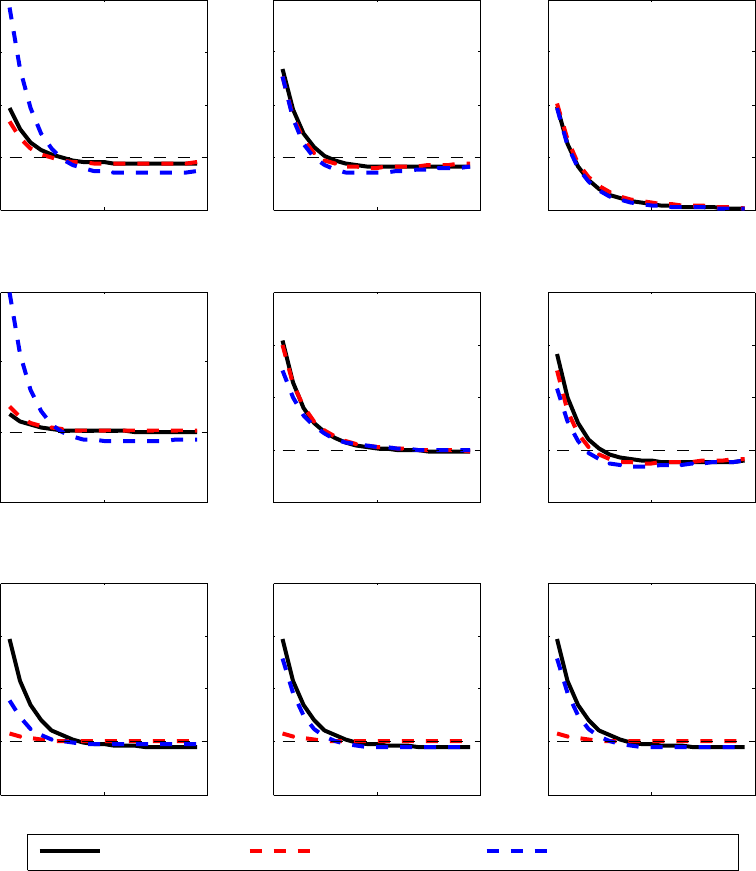
increase-related income. It is therefore crucial that in the case of more rigid wages of the poor

the increase in employment is strong enough to dominate the lower increase in wages. Note

also that the wealth effect on labour supply also works against the ampliﬁcation. However,

because the supply of searchers also depends on matching probability (and not only on

wages), the reduction in the number of searchers due to the wealth effect is not strong enough

to undo the effects of higher labour demand.

Figure 11: Effectiveness of monetary policy by groups (1)

0 10 20

−0.5

0.5

1.5

Consumption

Poor

0 10 20

−0.2

0.2

0.4

0.6

Middle

0 10 20

0.2

0.4

0.6

0.8

Rich

0 10 20

−1

Labour

0 10 20

−0.2

0.2

0.4

0.6

0 10 20

−0.2

0.2

0.4

0.6

0 10 20

−0.2

0.2

0.4

0.6

Wages

0 10 20

−0.2

0.2

0.4

0.6

0 10 20

−0.2

0.2

0.4

0.6

Flexible wages Sticky wages − all Sticky wages − poor

Notes: All variables are reported in percent deviations from the steady state. Units on the horizontal

axis are quarters.

ECB Working Paper Series No 2850

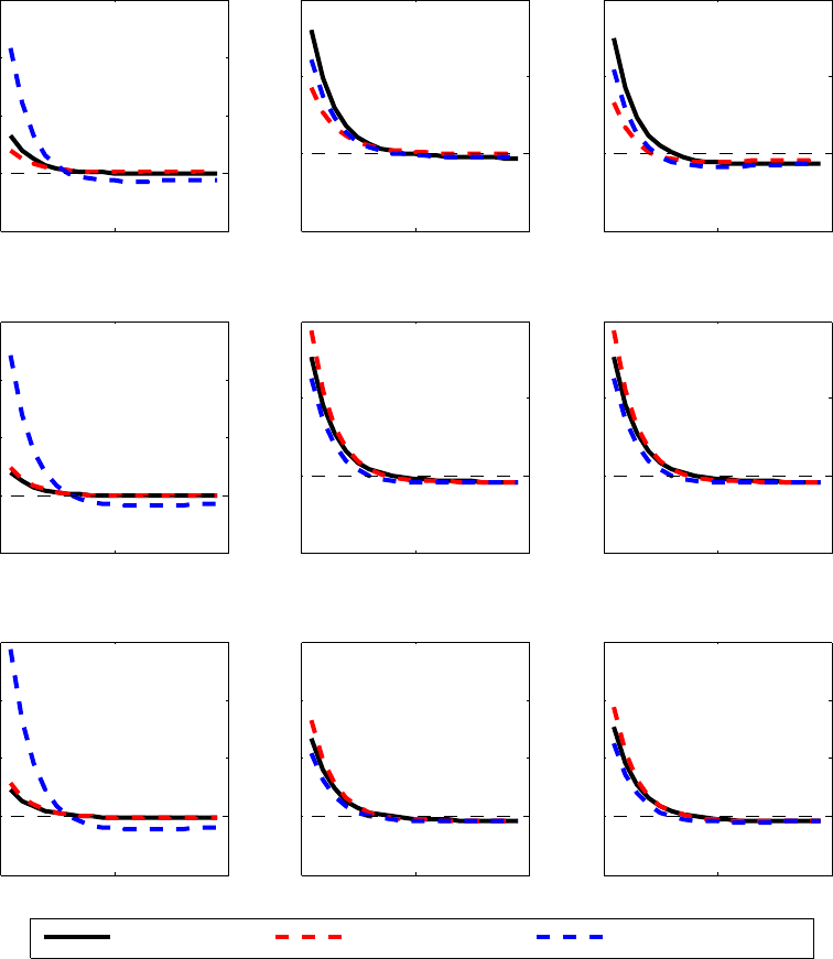
Figure 12: Effectiveness of monetary policy by groups (2)

0 10 20

−1

Labour income

Poor

0 10 20

−0.5

0.5

Middle

0 10 20

−0.5

0.5

Rich

0 10 20

−2

Tightness

0 10 20

−0.5

0.5

0 10 20

−0.5

0.5

0 10 20

−0.5

0.5

1.5

Prob.−worker

0 10 20

−0.2

0.2

0.4

0.6

0 10 20

−0.2

0.2

0.4

0.6

Flexible wages Sticky wages − all Sticky wages − poor

Notes: All variables are reported in percent deviations from the steady state. Units on the horizontal

axis are quarters.

ECB Working Paper Series No 2850

5 Conclusion

This paper ﬁrst documents several empirical characteristics of the labour market across ed-

ucational attainment levels. We ﬁnd that in several large European countries labour market

at low educational attainment levels is typically more precarious, with lower job ﬁnding

rates than those for high educational attainment. Moreover, job ﬁnding rates for low ed-

ucational attainment are typically also more volatile and more procyclical, which indicates

higher labour income risk in this segment of the labour market. At cyclical frequencies, ﬂuc-

tuations in job ﬁnding rates explain the majority of cyclical ﬂuctuations in unemployment

at the lower educational attainment levels, and the share of explained ﬂuctuations can ex-

ceed 80% in countries such as Germany and France. Cyclical ﬂuctuations in separation rates

tend to be less important in explaining ﬂuctuations in unemployment, especially at lower

educational attainment levels. The situation is similar in the US.

We then construct a stylised incomplete markets model with the search-and-matching

framework for segmented labour markets for workers with different educational attainment.

We calibrate the model to capture the characteristics that are in line with the empirical ﬁnd-

ings for Germany, Spain, and the US. We then use the differences to illustrate the transmission

channels of standard monetary policy in the model, and extend the analysis to forward guid-

ance.

Our main ﬁnding is that the effectiveness of monetary policy on consumption and output

is ampliﬁed if less educated and hence poorer households tend to obtain relatively more jobs

than more educated and richer households after a monetary stimulus. This result is only in

part due to the fact that poor households have the largest marginal propensities to consume.

There is also a general-equilibrium effect from higher aggregate consumption and output that

leads to more labour demand. When labour markets of the poor are more cyclical, this leads

to more hiring in these segments, which ampliﬁes the income and consumption of the poor

households and hence aggregate consumption. There may be several reasons that amplify

this transmission channel, either higher wage rigidity in the labour market segment for the

poor, or lower and hence more volatile proﬁts for hiring a worker from a less skilled labour

market segment, or both.

ECB Working Paper Series No 2850

References

(2016): “The Household Finance and Consumption Survey: results from the second wave,”

ECB Statistics Paper 18, Frankfurt a. M.

Acharya, S. and K. Dogra (2018): “Understanding HANK: insights from a PRANK,” Staff

Reports 835, Federal Reserve Bank of New York.

Adrjan, P. (2019): “What Next for British Steel Employees?” blog entry.

Amberg, N., T. Jansson, M. Klein, and A. R. Picco (2022): “Five Facts about the Distribu-

tional Income Effects of Monetary Policy Shocks,” American Economic Review: Insights, 4,

289–304.

Auclert, A. (2019): “Monetary policy and the redistribution channel,” American Economic

Review, 109, 2333–67.

Auclert, A. and M. Rognlie (2018): “Inequality and Aggregate Demand,” Working Paper

24280, National Bureau of Economic Research.

Bilbiie, F. (2018): “Monetary Policy and Heterogeneity: An Analytical Framework,” CEPR

Discussion Papers 12601, C.E.P.R. Discussion Papers.

Broer, T., N.-J. H. Hansen, P. Krusell, and E.

Oberg (2018): “The New Keynesian Trans-

mission Mechanism: A Heterogeneous-Agent Perspective,” .

Broer, T., J. Kramer, and K. Mitman (2022): “The Curious Incidence of Monetary Policy

Shocks Across the Income Distribution,” Sveriges Riksbank Working Paper, 416.

Daly, M. C., B. Hobijn, and T. S. Wiles (2012): “Dissecting aggregate real wage ﬂuctua-

tions: Individual wage growth and the composition effect,” Federal Reserve Bank of San

Francisco.

Den Haan, W. J., P. Rendahl, and M. Riegler (2017): “Unemployment (fears) and deﬂa-

tionary spirals,” Journal of the European Economic Association, 16, 1281–1349.

Den Haan, W. J. and P. Sedlacek (2014): “Inefﬁcient continuation decisions, job creation

costs, and the cost of business cycles,” Quantitative Economics, 5, 297–349.

Dolado, J. J., G. Motyovszki, and E. Pappa (2021): “Monetary policy and inequality un-

der labor market frictions and capital-skill complementarity,” American Economic Journal:

Macroeconomics, 13, 292–332.

Doniger, C. L. (2019): “Do Greasy Wheels Curb Inequality?” Finance and Economics Dis-

cussion Series 2019-021, Board of Governors of the Federal Reserve System (US).

Dossche, M. and J. Hartwig (2019): “Household Income Risk over the Business Cycle,”

Economic Bulletin, 6, 58–65.

ECB Working Paper Series No 2850

Elsby, M. W., B. Hobijn, and A. Sahin (2010): “The Labor Market in the Great Recession,”

Working Paper 15979, National Bureau of Economic Research.

Elsby, M. W., B. Hobijn, and A. S¸ahin (2013): “Unemployment dynamics in the OECD,”

Review of Economics and Statistics, 95, 530–548.

Elsby, M. W., B. Hobijn, and A. S¸ahin (2015): “On the importance of the participation

margin for labor market ﬂuctuations,” Journal of Monetary Economics, 72, 64 – 82.

Floden, M. and J. Lind

e (2001): “Idiosyncratic risk in the United States and Sweden: Is there

a role for government insurance?” Review of Economic dynamics, 4, 406–437.

Fujita, S. and G. Ramey (2009): “The cyclicality of separationa nd job ﬁnding rates,” Interna-

tional Economic Review, 50, 415–430.

Gornemann, N., K. Kuester, and M. Nakajima (2016): “Doves for the rich, hawks for the

poor? Distributional consequences of monetary policy,” .

Guvenen, F., S. Schulhofer-Wohl, J. Song, and M. Yogo (2017): “Worker Betas: Five Facts

about Systematic Earnings Risk,” American Economic Review, 107, 398–403.

Haefke, C., M. Sonntag, and T. van Rens (2013): “Wage rigidity and job creation,” Journal

of Monetary Economics, 60, 887 – 899.

Hagedorn, M., J. Luo, I. Manovskii, and K. Mitman (2018): “Forward Guidance,” Working

Paper 24521, National Bureau of Economic Research.

Hagedorn, M. and I. Manovskii (2008): “The cyclical behavior of equilibrium unemploy-

ment and vacancies revisited,” American Economic Review, 98, 1692–1706.

Hall, R. E. (2005): “Employment ﬂuctuations with equilibrium wage stickiness,” American

Economic Review, 95, 50–65.

Haltiwanger, J., H. Hyatt, and E. McEntarfer (2018): “Who Moves Up the Job Ladder?”

Journal of Labor Economics, 36, S301 – S336.

Hoynes, H., D. L. Miller, and J. Schaller (2012): “Who Suffers during Recessions?” Journal

of Economic Perspectives, 26, 27–48.

Kaplan, G., B. Moll, and G. L. Violante (2018): “Monetary Policy According to HANK,”

American Economic Review, 108, 697–743.

Kramer, J. (2022): “The Cyclicality of Earnings Growth along the Distribution-Causes and

Consequences,” mimeo.

Kudlyak, M. (2014): “The cyclicality of the user cost of labor,” Journal of Monetary Economics,

68, 53 – 67.

ECB Working Paper Series No 2850

Lenza, M. and J. Slacalek (2018): “How does monetary policy affect income and wealth

inequality? Evidence from quantitative easing in the euro area,” Working Paper Series

2190, European Central Bank.

McKay, A., E. Nakamura, and J. Steinsson (2016): “The Power of Forward Guidance Re-

visited,” American Economic Review, 106, 3133–58.

McKay, A. and R. Reis (2016): “The Role of Automatic Stabilizers in the U.S. Business Cycle,”

Econometrica, 84, 141–194.

Mueller, A. I. (2017): “Separations, Sorting, and Cyclical Unemployment,” American Eco-

nomic Review, 107, 2081–2107.

Patterson, C. (2023): “The Matching Multiplier and the Ampliﬁcation of Recessions,” Amer-

ican Economic Review, 113, 982–1012.

Petrongolo, B. and C. A. Pissarides (2001): “Looking into the black box: A survey of the

matching function,” Journal of Economic Literature, 39, 390–431.

Ravn, M. O. and V. Sterk (2016): “Macroeconomic Fluctuations with HANK & SAM: An

Analytical Approach,” Discussion Papers 1633, Centre for Macroeconomics (CFM).

——— (2017): “Job uncertainty and deep recessions,” Journal of Monetary Economics, 90, 125–

141.

Shimer, R. (2005): “The cyclical behavior of equilibrium unemployment and vacancies,”

American Economic Review, 95, 25–49.

——— (2012): “Reassessing the ins and outs of unemployment,” Review of Economic Dynamics,

15, 127–148.

Slacalek, J., O. Tristani, and G. L. Violante (2020): “Household balance sheet channels of

monetary policy: A back of the envelope calculation for the Euro Area,” Journal of Economic

Dynamics and Control, 115, 103879.

Werning, I. (2015): “Incomplete Markets and Aggregate Demand,” Working Paper 21448,

National Bureau of Economic Research.

ECB Working Paper Series No 2850

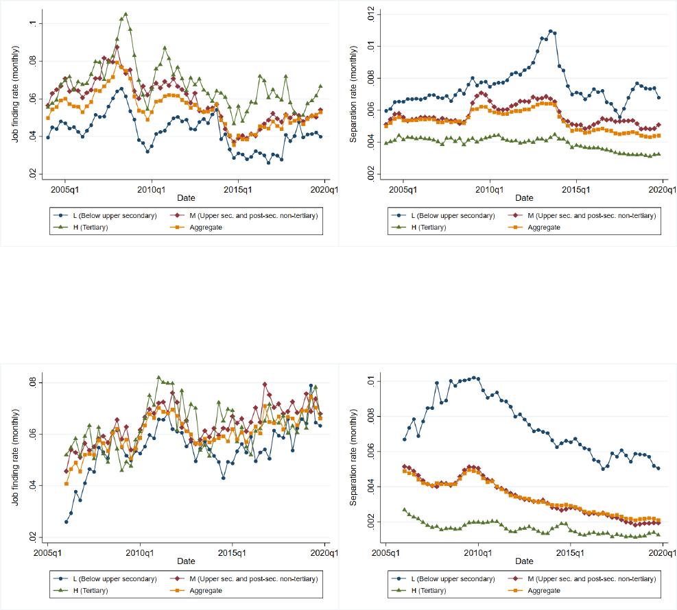
A Additional empirical evidence from European countries

A.1 Job ﬁnding rates and separation rates by educational attainment in

Europe

A.1.1 Unemployment duration spell less than 3 months (d<3)

Figure 13: France

Figure 14: Germany

ECB Working Paper Series No 2850

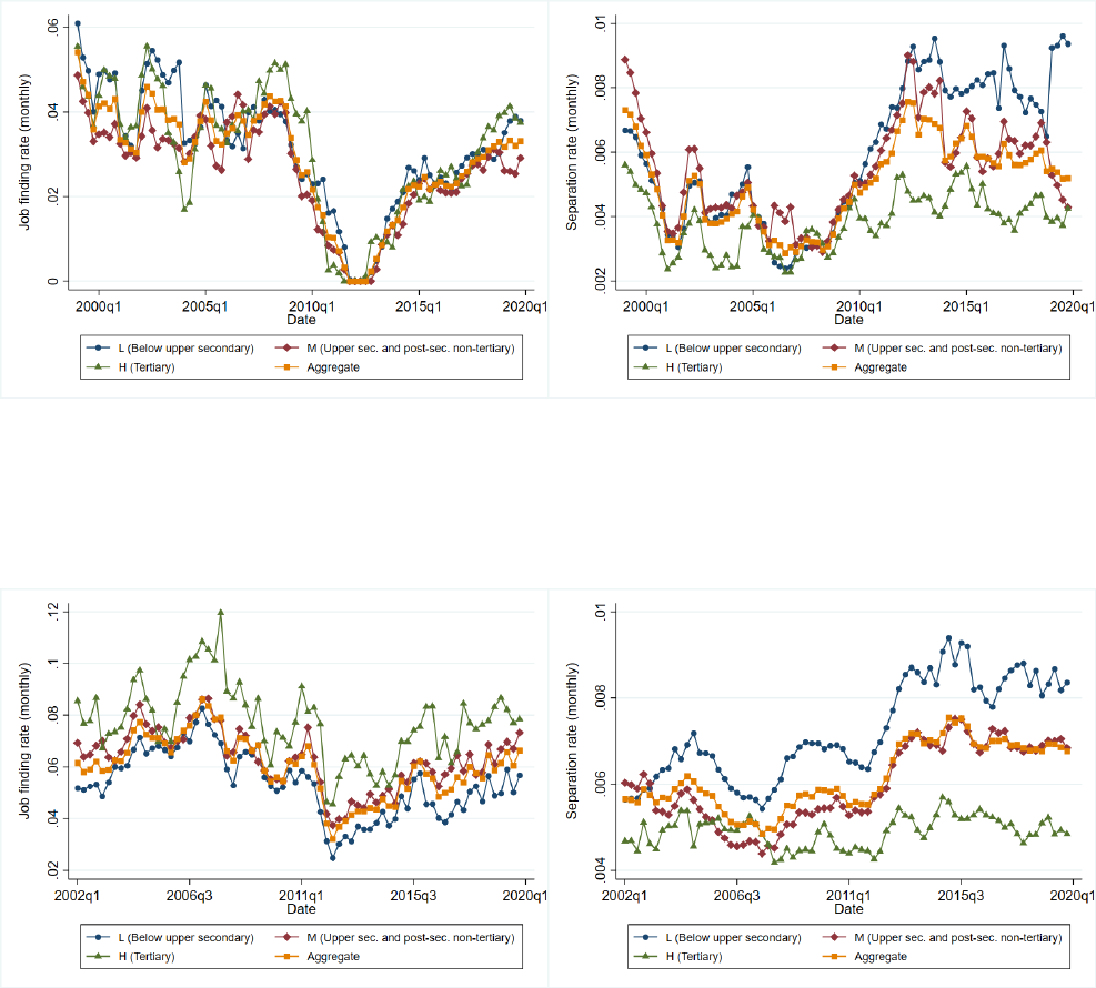
Figure 15: Greece

Figure 16: Italy

ECB Working Paper Series No 2850

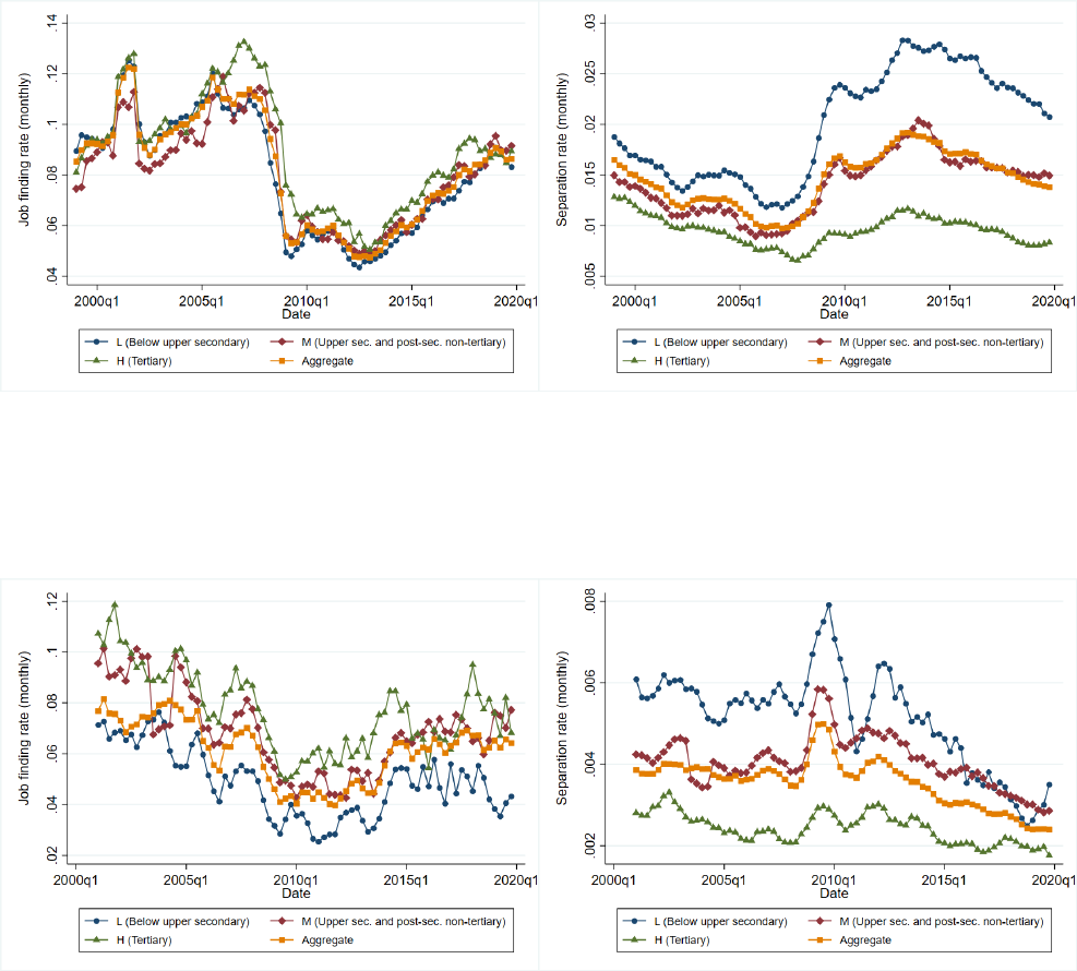
Figure 17: Spain

Figure 18: UK

ECB Working Paper Series No 2850

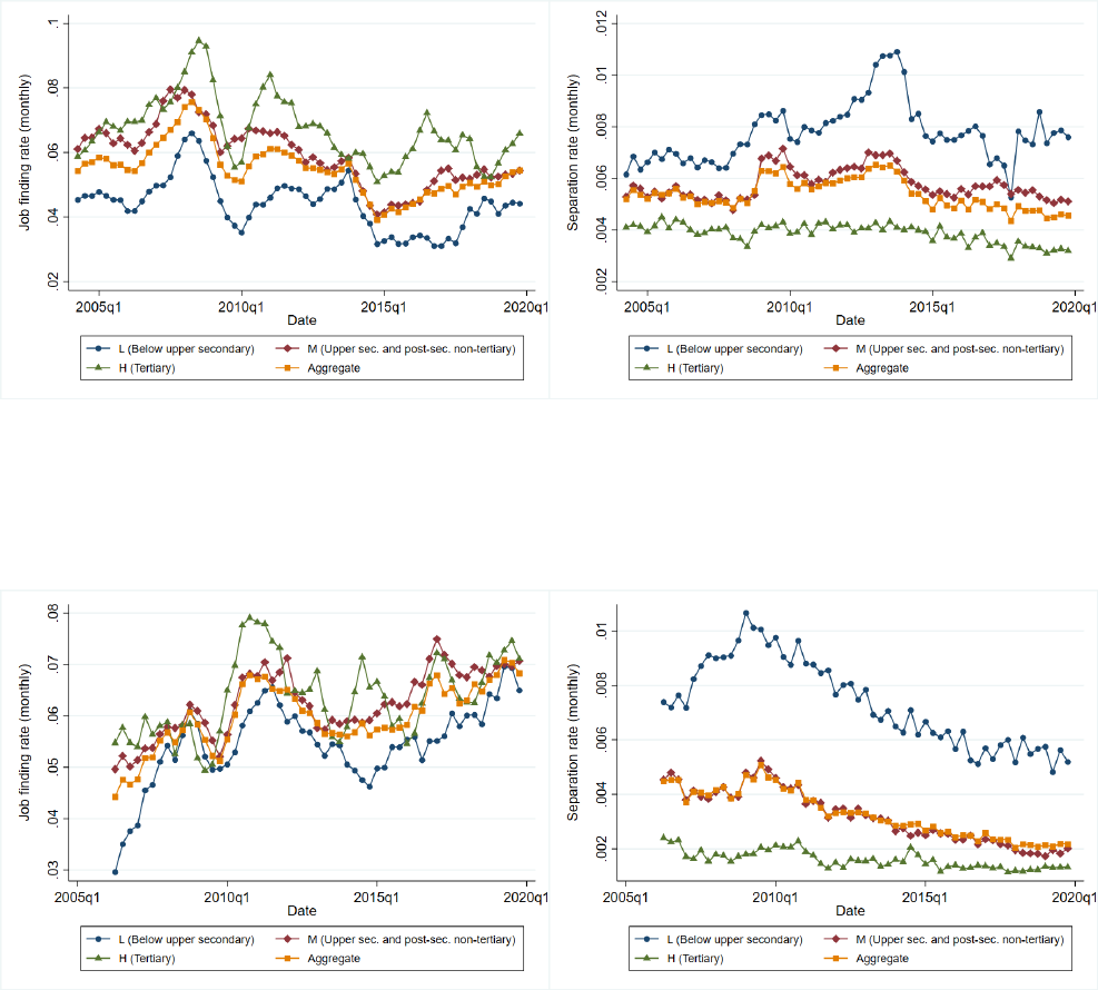
A.1.2 Unemployment duration spell less than 6 months (d<6)

Figure 19: France

Figure 20: Germany

ECB Working Paper Series No 2850

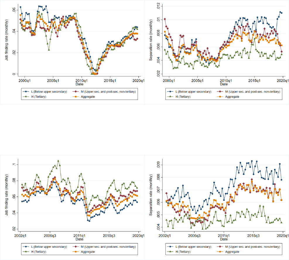
Figure 21: Greece

Figure 22: Italy

ECB Working Paper Series No 2850

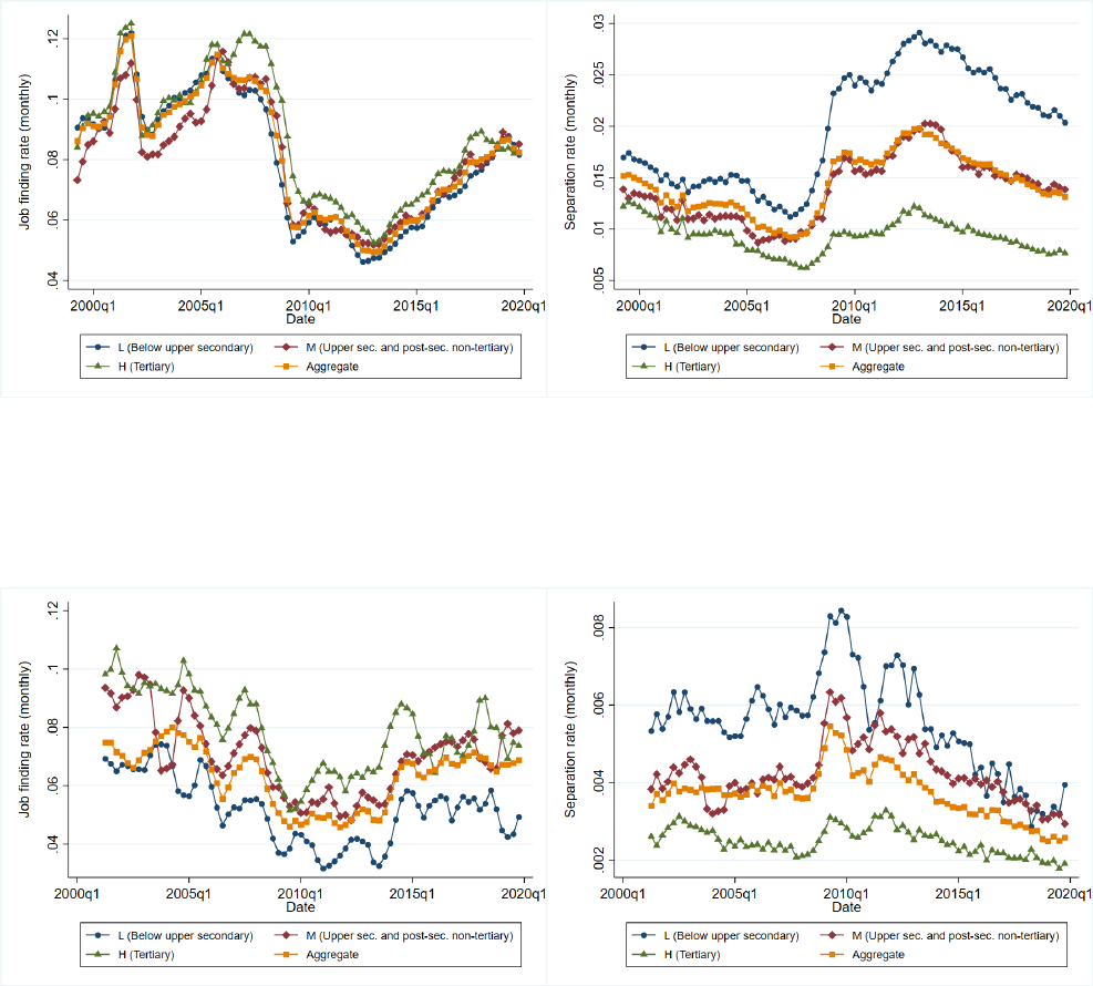
Figure 23: Spain

Figure 24: UK

ECB Working Paper Series No 2850

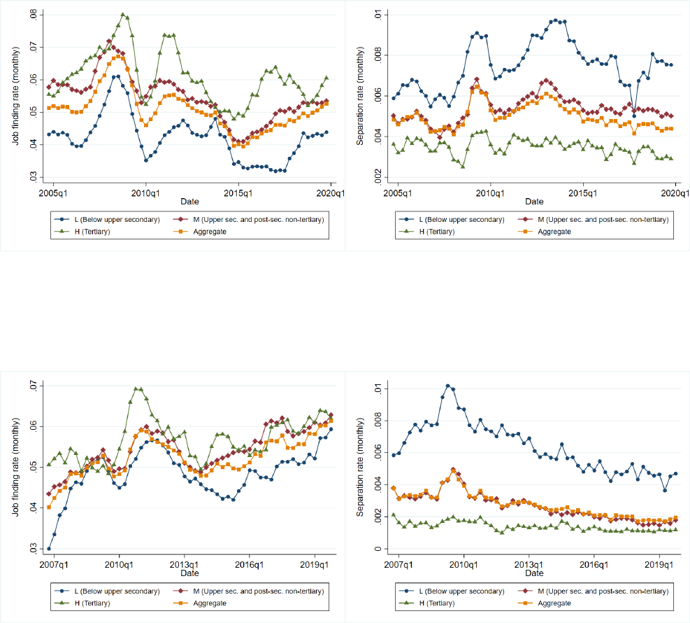
A.1.3 Unemployment duration spell less than 12 months (d<12)

Figure 25: France

Figure 26: Germany

ECB Working Paper Series No 2850

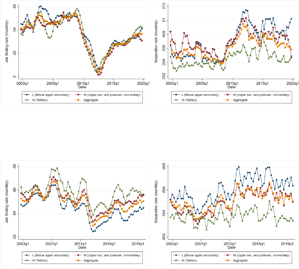
Figure 27: Greece

Figure 28: Italy

ECB Working Paper Series No 2850

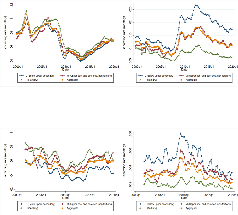
Figure 29: Spain

Figure 30: UK

ECB Working Paper Series No 2850

A.2 Job ﬁnding probabilities and separation probabilities across Euro-

pean countries

While the main text reports monthly job ﬁnding rates to be consistent with the literature

(e.g., Fujita and Ramey (2009), Shimer (2012)), it is sometimes convenient to have quarterly

probabilities, in particular, when calibrating models that are typically at a quarterly frequency.

This appendix reports the companion set of business cycle statistics in terms of quarterly

probabilities.

Table 12: Quarterly job ﬁnding probabilities

<12

Country Sample L M H L M H L M H

France 2003Q1-2019Q4 0.12 0.16 0.18 0.12 0.16 0.18 0.12 0.15 0.17

Germany 2005Q1-2019Q4 0.15 0.17 0.17 0.15 0.17 0.17 0.14 0.15 0.16

Greece 1998Q1-2019Q4 0.09 0.08 0.09 0.11 0.10 0.10 0.11 0.10 0.10

Italy 2001Q1-2019Q4 0.15 0.17 0.21 0.15 0.17 0.20 0.13 0.15 0.16

Spain 1998Q1-2019Q4 0.22 0.22 0.23 0.21 0.21 0.23 0.18 0.19 0.20

UK 2000Q1-2019Q4 0.14 0.19 0.21 0.15 0.19 0.21 0.13 0.18 0.18

Notes: The table reports quarterly job ﬁnding probabilities associated with the estimated monthly job ﬁnding

rates f

, computed as F

= 1 − e

−3 f

, where F

is the probability that an unemployed worker ﬁnds a job in

the next quarter. L = Less than primary, primary, and lower secondary education, M = Upper secondary and

post-secondary non-tertiary education, and H = Tertiary education. Values are sample averages. We end the

sample in Q4 2019 to exclude the COVID-19 period.

Table 13: Quarterly separation probabilities

<12

Country Sample L

M H L M H L M H

France 2003Q1-2019Q4 0.020 0.017

0.012 0.021 0.017 0.012 0.020 0.016 0.011

Germany 2005Q1-2019Q4 0.021 0.010 0.005 0.021 0.010 0.005 0.018 0.008 0.004

Greece 1998Q1-2019Q4 0.015 0.017 0.012 0.019 0.021 0.014 0.018 0.021 0.014

Italy 2001Q1-2019Q4 0.021 0.018 0.015 0.021 0.018 0.015 0.018 0.015 0.012

Spain 1998Q1-2019Q4 0.057 0.042 0.029 0.057 0.042 0.029 0.049 0.036 0.025

UK 2000Q1-2019Q4 0.015 0.012 0.008 0.016 0.013 0.008 0.014 0.011 0.007

Notes: The table reports quarterly separation probabilities associated with the estimated monthly separation

rates s

, computed as S

= 1 − e

−3s

, where S

is the probability that an employed worker loses a job in the

quarter. L = Less than primary, primary, and lower secondary education, M = Upper secondary and post-

secondary non-tertiary education, and H = Tertiary education. Values are sample averages. We end the sample

in Q4 2019 to exclude the COVID-19 period.

While quantitatively not important, note that the transformation from monthly rates to quarterly probabili-

ties is nonlinear. If x is rate and X is probability, the formula is X = 1 − e

−3x

ECB Working Paper Series No 2850

Table 14: Cyclical properties of job ﬁnding probabilities, quarterly

Rel.

own v

ol. Rel. aggregate vol. Corr. with agg.

σ(F

)/σ(U

) σ(F

)/σ(U) unemployment

Countr

y Sample L

M H L M H L M H

France

2003Q1-2019Q4 36.54 28.35

34.13 39.25 29.42 45.72 -0.60 -0.43 -0.55

Germany 2005Q1-2019Q4 42.06 31.02 39.72 40.40 34.50 56.94 -0.46 -0.20 -0.07

Greece 1998Q1-2019Q4 22.23 16.55 25.22 21.31 17.79 26.71 -0.40 -0.43 -0.42

Italy 2001Q1-2019Q4 29.32 30.17 39.44 30.47 29.97 45.36 -0.23 -0.41 -0.49

Spain 1998Q1-2019Q4 19.64 24.11 24.22 20.93 22.66 24.13 -0.61 -0.71 -0.81

UK 2000Q1-2019Q4 33.17 29.69 26.77 29.56 33.31 36.80 -0.33 -0.44 -0.30

Notes: The table reports standard deviations of cyclical components of quarterly job ﬁnding probabilities,

computed as F

= 1 − e

−3 f

, relative to the standard deviation of the cyclical component of each group’s un-

employment U

, aggregate unemployment U, and correlations of cyclical components of quarterly job ﬁnding

probabilities with the cyclical component of aggregate unemployment, all based on d = 3 estimates. L = Less

than primary, primary, and lower secondary education, M = Upper secondary and post-secondary non-tertiary

education, and H = Tertiary education. We end the sample in Q4 2019 to exclude the COVID-19 period.

Table 15: Cyclical properties of separation probabilities, quarterly

Rel. own vol. Rel. aggregate vol. Corr. with agg.

σ(S

)/σ(U

) σ(S

)/σ(U) unemployment

Country Sample L M H L M H L M H

France 2003Q1-2019Q4 3.00 2.43 0.86 3.22 2.53 1.15 -0.07 0.09 0.31

Germany 2005Q1-2019Q4 4.31 2.20 0.95 4.14 2.45 1.36 0.01 0.65 0.52

Greece 1998Q1-2019Q4 2.09 2.67 1.72 2.00 2.88 1.83 0.31 0.25 0.10

Italy 2001Q1-2019Q4 1.91 1.52 1.31 1.98 1.51 1.50 0.67 0.60 0.39

Spain 1998Q1-2019Q4 3.63 2.68 1.47 3.87 2.52 1.46 0.83 0.81 0.81

UK 2000Q1-2019Q4 2.40 1.48 0.82 2.14 1.66 1.13 0.23 0.47 0.66

Notes: The table reports standard deviations of cyclical components of quarterly separation probabilities, com-

puted as S

= 1 − e

−3s

, relative to the standard deviation of the cyclical component of each group’s unemploy-

ment U

, aggregate unemployment U, and correlations of cyclical components of quarterly separation prob-

abilities with the cyclical component of aggregate unemployment, all based on d = 3 estimates. L = Less

than primary, primary, and lower secondary education, M = Upper secondary and post-secondary non-tertiary

education, and H = Tertiary education. We end the sample in Q4 2019 to exclude the COVID-19 period.

ECB Working Paper Series No 2850

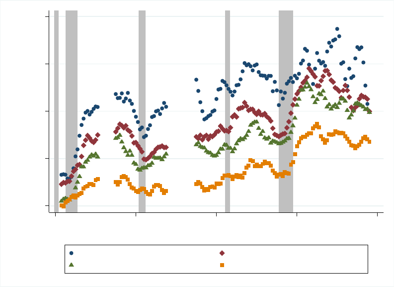
B Additional empirical evidence from the US

B.1 Wage rigidity in the US

Figure 31: Wage rigidity by educational attainment – Full sample

5 10 15 20 25

Nominal wage rigidity

1980q1 1990q1 2000q1 2010q1 2020q1

date

Less than high school High school or equivalent, no college

Some college or Associate degree Bachelor’s or advanced degree

Notes: Percentage of workers who saw no change in their wage over the past year by educational attainment.

Source: https://www.frbsf.org/economic-research/indicators-data/nominal-wage-rigidity/

ECB Working Paper Series No 2850

B.2 Alternative measures of a business cycle

Table 16: Worker ﬂows over business cycle

(1)

(2) (3)

Net hir

es Hires Separations

NBER

recession -0.013*** -0.015***

-0.004

(0.001) (0.002) (0.003)

Less than high school 0.001*** 0.030*** 0.029***

(0.000) (0.001) (0.001)

High school or equivalent, no college -0.001*** 0.011*** 0.012***

(0.000) (0.000) (0.000)

Some college or Associate degree -0.000 0.006*** 0.006***

(0.000) (0.000) (0.000)

Less than high school × NBER recession -0.007*** 0.002* 0.008***

(0.001) (0.001) (0.001)

High school or equivalent, no college × NBER recession -0.003*** -0.000 0.003***

(0.001) (0.001) (0.001)

Some college or Associate degree × NBER recession -0.002** -0.000 0.001*

(0.001) (0.001) (0.001)

ime FE X X

Observations 272 276 276

R-squared 0.929 0.971 0.954

Robust

standard err

ors in parentheses

*** p<0.01, ** p<0.05, * p<0.1

Notes: (Net) hires and separations are rates and are expressed as a share of average employment within the

education group. NBER recession is a dummy variable indicating NBER recessions.

ECB Working Paper Series No 2850

Table 17: Worker ﬂows over the business cycle

(1)

(2) (3)

Net hir

es Hires Separations

Less

than high school 0.000

0.030*** 0.030***

(0.000) (0.001) (0.001)

High school or equivalent, no college -0.001*** 0.011*** 0.012***

(0.000) (0.000) (0.000)

Some college or Associate degree -0.001** 0.006*** 0.007***

(0.000) (0.000) (0.000)

Less than high school × UE cycle -0.007** -0.006* 0.001

(0.003) (0.003) (0.005)

High school or equivalent, no college × UE cycle -0.004** -0.000 0.004

(0.002) (0.002) (0.002)

Some college or Associate degree × UE cycle -0.002 0.000 0.003

(0.002) (0.002) (0.002)

ime FE X X

Observations 272 276 276

R-squared 0.895 0.971 0.947

Robust

standard err

ors in parentheses

*** p<0.01, ** p<0.05, * p<0.1

Notes: (Net) hires and separations are rates and are expressed as a share of an average employment within

the education group. UE cycle is the cyclical component of unemployment level within the educational group,

obtained by the Hodrick-Prescott Filter using logarithm of seasonally adjusted unemployment level.

ECB Working Paper Series No 2850

B.3 Sensitivity of ﬂows to changes in the GDP

To estimate the sensitivity of changes in (net) hires and separation rates to changes in the

GDP across education groups, we estimate the following speciﬁcation:

∆Y

i,t

= γ

+ θ

educ

+ θ

educ

× ∆lnGDP

+ ϵ

i,t

, (37)

where ∆Y

i,t

is the change in either (net) hire or separation rate, educ

is workers’ educational

attainment, ∆lnGDP

is the change in the logarithm of GDP, γ

are time dummies to control

for common shocks, and ϵ

i,t

is the residual term.

Table 18: Sensitivity of worker ﬂows to changes in GDP

(1) (2) (3)

∆ Net hires ∆ Hir

es ∆ Separations

Less than high school -0.0007*

-0.0007*** -0.0001

(0.0003) (0.0003) (0.0002)

High school or equivalent, no college -0.0003 -0.0002 0.0000

(0.0003) (0.0002) (0.0002)

Some college or Associate degree -0.0002 -0.0001 0.0001

(0.0003) (0.0002) (0.0002)

Less than high school * ∆ ln GDP 0.1505*** 0.0937** -0.0542*

(0.0431) (0.0370) (0.0312)

High school or equivalent, no college * ∆ ln GDP 0.0767** 0.0429* -0.0309

(0.0305) (0.0227) (0.0252)

Some college or Associate degree * ∆ ln GDP 0.0489 0.0210 -0.0264

(0.0329) (0.0279) (0.0245)

Time FE X X X

Obser

vations 268 272 272

R-squared 0.8720 0.8017 0.8673

Robust standard err

ors in parentheses

*** p<0.01, ** p<0.05, * p<0.1

ECB Working Paper Series No 2850

C The remaining model equations

This section describes the remaining model equations. The description closely follows McKay

et al. (2016).

Final goods and intermediate goods. Final goods Y

are produced by bundling intermedi-

ate goods y

j,t

, using



j,t



(38)

Intermediate goods are produced by a continuum of mass 1 of intermediate goods ﬁrms

indexed by j according to the following technology:

j,t

= n

j,t

, (39)

where n

j,t

is the amount of labour services hired by the intermediate goods ﬁrm j. The ﬁnal

good is produced by a representative competitive ﬁrm, but intermediate goods are produced

by monopolistically competitive ﬁrms. These ﬁrms are subject to pricing frictions and can

update their prices only with a probability θ per period. The optimisation of the ﬁnal goods

producer implies

j,t



j,t



1−µ

, (40)

where p

j,t

is the price charged by ﬁrm j at time t and P

is the aggregate price level, given by



1−µ

j,t



1−µ

. (41)

The intermediate producer solves the following problem:

max

∗

,{y

j,s

}

∞

s=t

∞

∑

s=t

s−t

(1 − θ)

s−t



∗

j,s

− W

j,s



, (42)

subject to 39 and 40. The solution to this problem is

∗

∑

∞

s=t

s−t

(1 − θ)

s−t



∗



1−µ

µW

∑

∞

s=t

s−t

(1 − θ)

s−t



∗



1−µ

. (43)

Government. The government runs a balanced budget, using taxes levied based on (exoge-

nous) labour productivity only to pay interest on otherwise constant bond stock,

1 + r

∑

(z)τ

τ(z) = B (44)

The relation between nominal rate, real rate, and inﬂation is

ECB Working Paper Series No 2850

1 + r

1 + i

1 + π

t+1

. (45)

Equilibrium. In equilibrium, if Γ

(b, z) is the distribution of households asset holdings b

over the idiosyncratic state z at time t, that satisﬁes

t+1



B, z

′



{(b,z):g

(b,z)∈B}



′



dΓ

(b, z), (46)

where g

(b, z) is the decision rule for household’s savings.

Labour supply by households through labour ﬁrms has to be equal to labour demand by

intermediate goods ﬁrms:

≡

h,t

(b, z)dΓ

(b, z), (47)

where the aggregation is across household types and their labour supply (note that l

h,t

de-

pends both on household’s wealth and the matching probabilities across labour market seg-

ments). Labour market clearing implies

= N

. (48)

Aggregate production is

≡

j,t

dj = Y

, (49)

where S

is price dispersion due to nominal rigidities, deﬁned as

≡



j,t



dj (50)

with the law of motion

t+1

= (1 − θ)S

(1 + π

t+1

)

−µ

1−µ

+ θ



∗

t+1



1−µ

. (51)

Inﬂation can be deﬁned as

1 + π







1 − θ



∗



1−µ







1−µ

. (52)

In addition, labour markets clear, bond markets clear, and goods markets clear (taking into

account that dividends are D

= Y

− W

)

B =

(b, z)dΓ

(b, z), (53)

ECB Working Paper Series No 2850

= C

. (54)

In equilibrium, all decision rules, value functions satisfy all optimality conditions, deﬁnitions,

and budget constraints.

ECB Working Paper Series No 2850

D Forward guidance and labour market volatility

D.1 European countries

For completeness, this appendix reports the implications of higher volatility on the labour

market for the poor on the effectiveness of forward guidance. We simulate forward guidance

as a fully credible announcement of a one-time interest rate decrease in period 10. The results

are reported in Figures 32 to 34, again for two cases: the red dashed line show our benchmark

case, where labour market for the poor is very volatile, and the full black lines show the case

where this volatility is smaller (but still higher than in the segments for the middle-income

and rich households).

ECB Working Paper Series No 2850

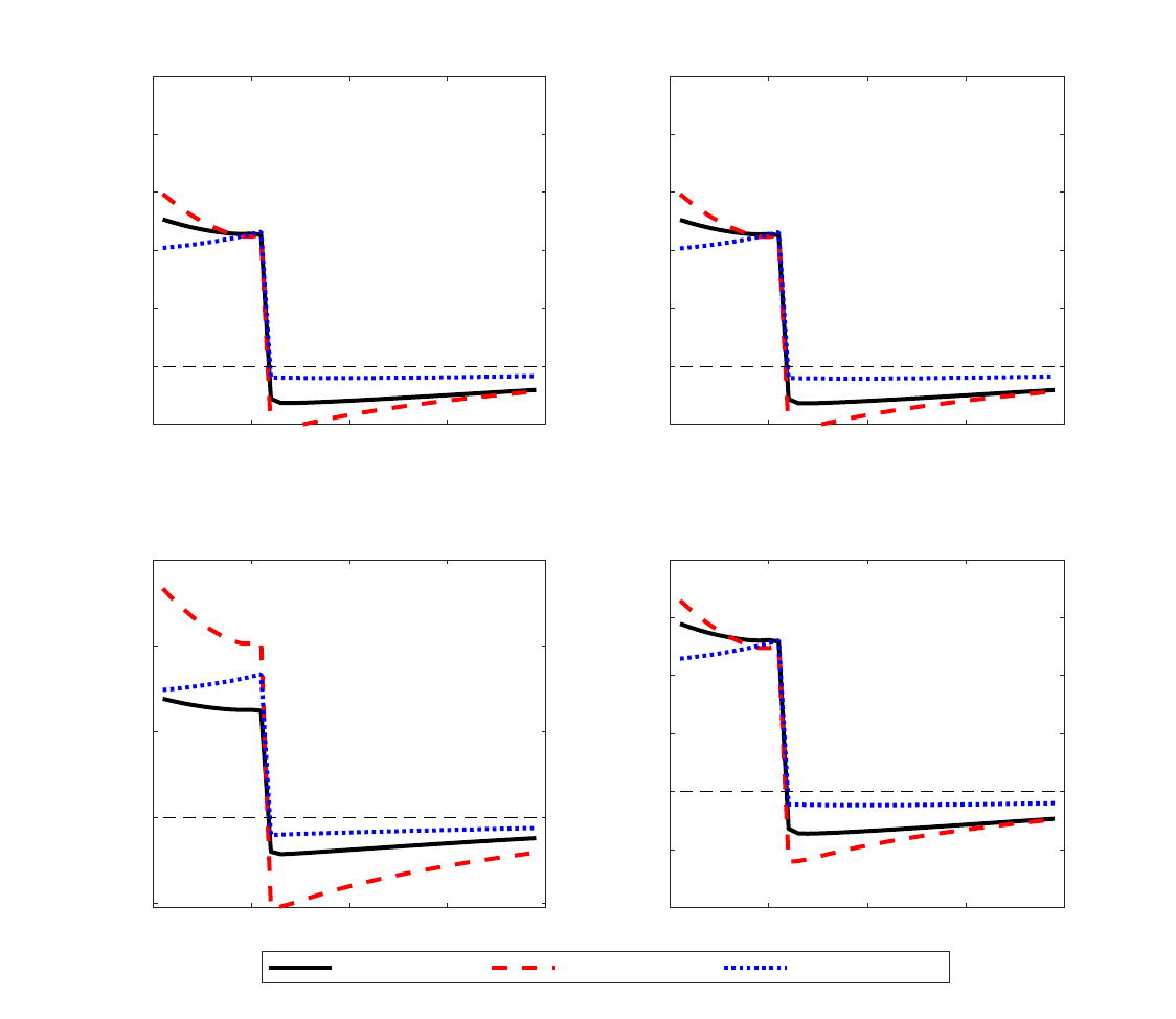
Figure 32: Effectiveness of forward guidance depending on who gets jobs

0 10 20 30 40

-0.1

0.1

0.2

0.3

0.4

0.5

Output (Consumption)

0 10 20 30 40

-0.1

0.1

0.2

0.3

0.4

0.5

Labour

0 10 20 30 40

-0.05

0.05

0.1

0.15

Dividends

0 10 20 30 40

-0.2

-0.1

0.1

0.2

0.3

0.4

Total labour income (pre-tax)

Poor less volatile Poor more volatile All equally volatile

Notes: All variables are reported in percent deviations from the steady state. Units on the horizontal

axis are quarters.

ECB Working Paper Series No 2850

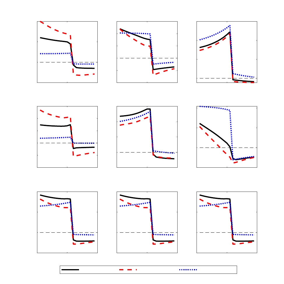
Figure 33: Effectiveness of forward guidance by groups (1)

0 10 20

-0.5

0.5

Consumption

Poor

0 10 20

-0.2

-0.1

0.1

0.2

0.3

Middle

0 10 20

0.1

0.2

0.3

Rich

0 10 20

-1

-0.5

0.5

1.5

Labour

0 10 20

-0.1

0.1

0.2

0.3

0 10 20

-0.1

0.1

0.2

0 10 20

-0.01

0.01

0.02

Wages

0 10 20

-0.01

0.01

0.02

0 10 20

-0.01

0.01

0.02

Poor less volatile Poor more volatile All equally volatile

Notes: All variables are reported in percent deviations from the steady state. Units on the horizontal

axis are quarters.

ECB Working Paper Series No 2850

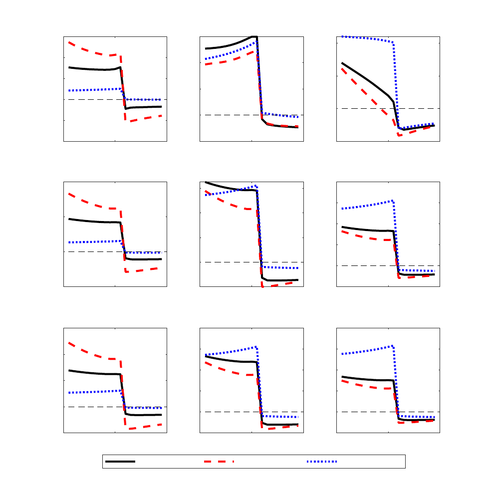
Figure 34: Effectiveness of forward guidance by groups (2)

0 10 20

-1

-0.5

0.5

1.5

Labour income

Poor

0 10 20

-0.1

0.1

0.2

0.3

Middle

0 10 20

-0.1

0.1

0.2

Rich

0 10 20

-2

Tightness

0 10 20

-0.2

0.2

0.4

0.6

0 10 20

-0.2

0.2

0.4

0.6

0.8

0 10 20

-0.1

0.1

0.2

0.3

Prob.-worker

0 10 20

-0.02

0.02

0.04

0.06

0.08

0 10 20

-0.02

0.02

0.04

0.06

0.08

Poor less volatile Poor more volatile All equally volatile

Notes: All variables are reported in percent deviations from the steady state, except probabilities,

which are in percentage points. Units on the horizontal axis are quarters.

D.2 Calibration to the US

This section reports the implications of different wage stickiness across labour market seg-

ments for the effectiveness of forward guidance. Similarly to standard monetary policy in the

main text, the effectiveness of forward guidance depends on who obtains jobs. As shown in

Figures 35, 36, and 37, the ampliﬁcation of the forward guidance ”puzzle” is mainly driven

by the poor obtaining jobs, i.e, the mechanisms at work are similar as for the standard mone-

tary policy shock described above. We obtain the ampliﬁcation of the strength of the forward

ECB Working Paper Series No 2850

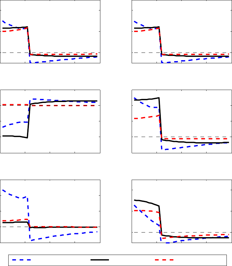
guidance only when the poor obtain jobs.

Figure 35: Forward guidance depending on who gets jobs

0 10 20 30 40

0.2

0.4

Output (Consumption)

0 10 20 30 40

0.2

0.4

Labour

0 10 20 30 40

−1.5

−1

−0.5

0.5

Dividends

0 10 20 30 40

−0.2

0.2

0.4

0.6

Total labour income (pre−tax)

0 10 20 30 40

−0.5

0.5

1.5

Labour by poor

0 10 20 30 40

0.2

0.4

Labour by rich

Sticky wages − poor Flexible wages Sticky wages − all

Notes: All variables are reported in percent deviations from the steady state. Units on the horizontal

axis are quarters.

ECB Working Paper Series No 2850

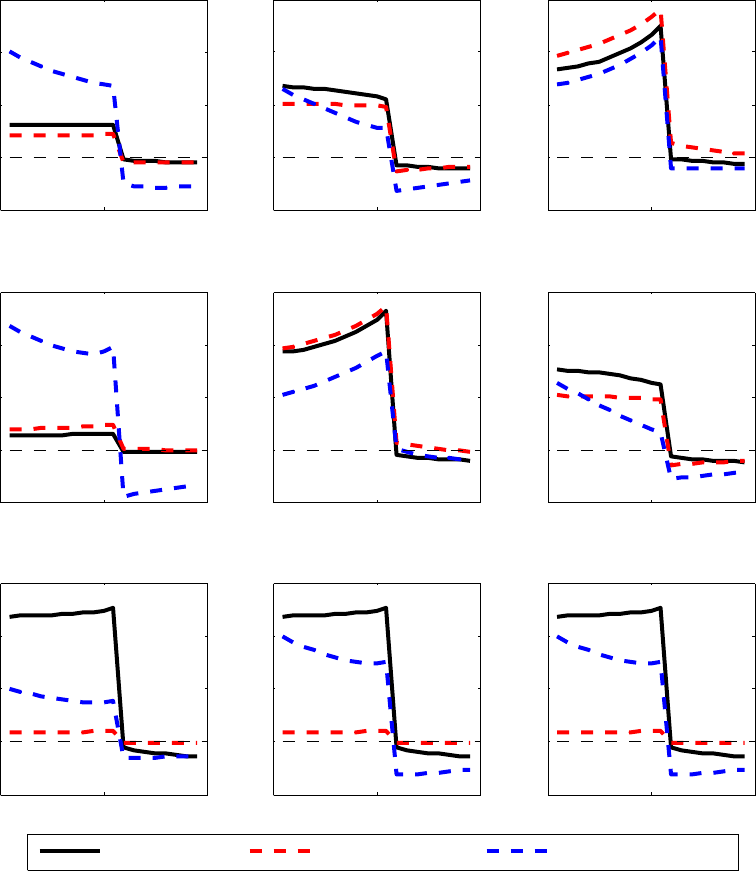
Figure 36: Forward guidance, by groups (1)

0 10 20

−0.5

0.5

1.5

Consumption

Poor

0 10 20

−0.2

0.2

0.4

0.6

Middle

0 10 20

−0.1

0.1

0.2

0.3

Rich

0 10 20

−0.5

0.5

1.5

Labour

0 10 20

−0.1

0.1

0.2

0.3

0 10 20

−0.2

0.2

0.4

0.6

0 10 20

−0.1

0.1

0.2

0.3

Wages

0 10 20

−0.1

0.1

0.2

0.3

0 10 20

−0.1

0.1

0.2

0.3

Flexible wages Sticky wages − all Sticky wages − poor

Notes: All variables are reported in percent deviations from the steady state. Units on the horizontal

axis are quarters.

ECB Working Paper Series No 2850

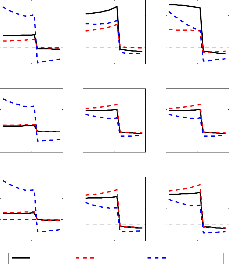
Figure 37: Forward guidance, by groups (2)

0 10 20

−0.5

0.5

1.5

Labour income

Poor

0 10 20

−0.2

0.2

0.4

0.6

Middle

0 10 20

−0.2

0.2

0.4

0.6

Rich

0 10 20

−2

Tightness

0 10 20

−0.5

0.5

0 10 20

−0.5

0.5

0 10 20

−0.5

0.5

Prob.−worker

0 10 20

−0.1

0.1

0.2

0.3

0 10 20

−0.1

0.1

0.2

0.3

Flexible wages Sticky wages − all Sticky wages − poor

Notes: All variables are reported in percent deviations from the steady state. Units on the horizontal

axis are quarters.

ECB Working Paper Series No 2850

Acknowledgements

We have benefited from conversations with Husnu Dalgic, Wouter den Haan, Francois Langot, Ralph Lütticke, Reamonn Lydon,

Benjamin Moll, Ricardo Reis, Petr Sedláček, Jirka Slačálek, Vincent Sterk, and Gianluca Violante. We are also grateful to seminar

participants in the 25th International CEF meeting, the Annual Workshop: ESCB Research Cluster 2 in Frankfurt, the conference on

Income Distribution, Wealth Distribution and Central Bank Policies in London (2020), 2020 Frankfurt – Mannheim Macro Workshop,

2020 Central Bank Macro Modelling Workshop, and RES 2021 Annual Conference.

The opinions expressed are those of the authors and do not reflect views of the European Central Bank or of the Eurosystem. Part of

this paper has been written while Matija was at the ECB. All errors are our own.

Uroš Herman

Aix Marseille University, CNRS, AMSE, Marseille, France; email: uros.herman@univ-amu.fr

Matija Lozej

Central Bank of Ireland, Dublin, Ireland; email: matija.lozej@centralbank.ie

Postal address 60640 Frankfurt am Main, Germany

Telephone +49 69 1344 0

Website www.ecb.europa.eu

electronically, in whole or in part, is permitted only with the explicit written authorisation of the ECB or the authors.

This paper can be downloaded without charge from www.ecb.europa.eu, from the Social Science Research Network electronic library or

from RePEc: Research Papers in Economics. Information on all of the papers published in the ECB Working Paper Series can be found

on the ECB’s website.

PDF ISBN 978-92-899-6215-5 ISSN 1725-2806 doi:10.2866/325480 QB-AR-23-087-EN-N