
This paper presents preliminary findings and is being distributed to economists
and other interested readers solely to stimulate discussion and elicit comments.
The views expressed in this paper are those of the authors and do not necessarily
reflect the position of the Federal Reserve Bank of New York or the Federal
Reserve System. Any errors or omissions are the responsibility of the authors.
Federal Reserve Bank of New York
Staff Reports
Optimal Monetary Policy
According to HANK
Sushant Acharya
Edouard Challe
Keshav Dogra
Staff Report No. 916
February 2020
Optimal Monetary Policy According to HANK
Sushant Acharya, Edouard Challe, and Keshav Dogra
Federal Reserve Bank of New York Staff Reports, no. 916
February 2020
JEL classification: E21, E30, E52, E62, E63
Abstract
We study optimal monetary policy in a heterogeneous agent new Keynesian economy. A
utilitarian
planner seeks to reduce consumption inequality, in addition to stabilizing output gaps
and inflation. The
planner does so both by reducing income risk faced by households, and by
reducing the pass-through from
income to consumption risk, trading off the benefits of lower
inequality against productive inefficiency
and higher inflation. When income risk is
countercyclical, policy curtails the fall in output in recessions
to mitigate the increase in
inequality. We uncover a new form of time inconsistency of the Ramsey plan—the temptation to
exploit households' unhedged interest rate exposure to lower inequality.
Key words: new Keynesian model, incomplete markets, optimal monetary policy
_________________
Acharya, Dogra: Federal Reserve Bank of New York (emails: sushant.acharya@ny.frb.org,
keshav.dogra@ny.frb.org). Challe: CREST and Ecole Polytechnique (email:
edouard.chal[email protected]). The authors thank Florin Bilbiie, Christopher Carroll, Russell
Cooper, Clodomiro Ferreira, Antoine Lepetit, Galo Nuño, Pedro Teles, Gianluca Violante, and
Pierre-Olivier Weil for helpful discussions. They also received useful comments from seminar
participants at HEC Paris, UT Austin, UC3M, EUI, Université Paris-Dauphine, Université Paris
8, Banque de France, and CREST, as well as from conference participants at the Barcelona GSE
Summer Forum (Monetary Policy and Central Banking), the NBER Summer Institute (Micro
Data and Macro Models), the Salento Macro Meetings, SED, and T2M. Edouard Challe
acknowledges financial support from the French National Research Agency (Labex
Ecodec/ANR-11-LABX-0047). The views expressed in this paper are those of the authors and do
not necessarily reflect the position of the Federal Reserve Bank of New York or the Federal
Reserve System.
To view the authors’ disclosure statements, visit
https://www.newyorkfed.org/research/staff_reports/sr916.html.
1 Introduction
It is increasingly recognized by researchers and policymakers that monetary policy can have important
effects on inequality. Despite this, the study of how monetary policy should be conducted optimally has
only recently begun to depart from a representative agent framework in which concerns about inequality
are trivially absent. While the large recent heterogeneous agent New Keynesian (HANK) literature has
shown that uninsurable idiosyncratic risk and inequality can dramatically change the positive effects of
monetary policy on the macroeconomy (See for example Ravn and Sterk (2017, Forthcoming); Kaplan et
al. (2018); den Haan et al. (2018); Auclert et al. (2018); Auclert (2019); Bilbiie (2019a) and many others),
the normative implications of HANK and the reciprocal effects of monetary policy on risk and inequality,
have been less well studied. This gap in the literature partly exists because characterizing optimal policy
in HANK economies is technically difficult. Solving for the Ramsey optimal policy involves choosing the
evolution of an infinite dimensional state variable (the wealth distribution), as well as infinite dimensional
controls (the distribution of consumption and hours worked across agents) subject to an infinite number
of constraints (each household’s optimality condition and budget constraints).
One approach to solving optimal policy problems for HANK economies is computational, and re-
searchers have recently started developing numerical algorithms to handle them (Bhandari et al., 2018).
We instead take an analytical approach. We study a standard NK economy with nominal rigidities with
the exception that households face uninsurable idiosyncratic risk. Markets are incomplete and agents can
only self-insure by trading a riskless bond or by working longer hours. We assume that households have
constant absolute risk (CARA) utility and idiosyncratic shocks are normally distributed. As in Acharya
and Dogra (2018), these assumptions imply that the economy permits linear aggregation which in turn
means that the infinite dimensional distributions of consumption, hours worked and wealth can be summa-
rized by their cross-sectional averages: the positive behavior of macroeconomic aggregates can be described
independently of the distribution of the wealth distribution. Of course, from a normative perspective, the
dispersion of wealth does affect social welfare and hence the optimal conduct of monetary policy. Crucially,
the effect of inequality on social welfare is also summarized by a finite dimensional sufficient statistic. This
makes the optimal policy problem analytically tractable, allowing us to drill down and identify exactly the
features that makes the optimal conduct of monetary policy different in HANK economies compared to
the RANK benchmark.
As is commonly known, in RANK the planner seeks to stabilize prices and keep output at its produc-
tively efficient level. In HANK, the planner has an additional objective - to use monetary policy to reduce
the cross-sectional consumption dispersion that results from the cumulated effects of uninsured idiosyn-
cratic shocks. This incentive is shut down in RANK by construction. We show that there are three ways in
which the planner can use monetary policy to achieve this purpose. First, the central bank may attempt
to reduce the amount of income risk that households are exposed to (the income risk channel). How to
achieve this reduction naturally depends on the cyclicality of income risk: if this risk is countercyclical,
then the central bank has an incentive to raise output in order to lower risk, while the opposite is true
if risk is procyclical. Either way, the central bank’s willingness and ability to manipulate the amount of
idiosyncratic risk that households face gives it an incentive to move output away from the level consistent
1

with stable prices and productive efficiency.
1
The second way in which the central bank may reduce consumption dispersion, independently of affect-
ing the level of income risk, is by reducing the pass-through from income risk to consumption risk, that is,
by lowering the marginal propensity to consume out of a change in individual income (the self-insurance
channel). This pass-through ultimately reflects the ability of the households to self-insure against idiosyn-
cratic risk through borrowing or working longer hours, and is thus affected by the paths of real interest
rates and wages going forward. On the one hand, lower interest rates make it easier for households to
borrow in response to an unfavorable shock, making individual consumption less response to changes in
individual income; this ultimately reduces consumption dispersion at any level of income risk. On the other
hand, higher wages going forward make it easier for households to buffer the impact of a fall in current
income on current consumption by borrowing today and working longer hours in the future to repay the
debt. When future wages are high, only a small increase in hours ( and hence the incurred dis-utility)
worked is required to repay this debt. This again makes individual consumption less responsive to changes
in current income. It follows that the central bank has an incentive to commit to low interest rates and
high wages –i.e., to be expansionary– going forward in order to reduce the pass-through from income risk
to consumption risk. This incentive is of course absent in RANK.
Finally, the central bank can reduce consumption dispersion through unanticipated changes in the
marginal propensity to consume out of wealth. Given a distribution of wealth, an unexpected fall in
interest rates benefits poor debtors, reducing their interest payments and increasing their consumption
(the unhedged interest rate exposure (URE) channel) (Auclert, 2019). Conversely, lower interest rates
reduce the interest income of rich savers, reducing their consumption. Overall, lower rates reduce the
marginal propensity to consume out of wealth, reducing consumption inequality. Importantly, this channel
(unlike the previous two) only operates for unexpected changes in interest rates, as we explain in more
detail in Section 4.
How does the presence of these three channels, through which the planner can affect inequality, change
the optimal conduct of monetary policy? As is commonly known, in RANK, optimal monetary policy
features divine coincidence in response to productivity shocks (Blanchard and Gal´ı, 2007): it is both
feasible and optimal to stabilize both the gap between output and its efficient level (output gap), and
inflation. In our RANK economy, in the empirically relevant case where income risk is countercyclical,
while it remains feasible to stabilize the output gap and inflation, it is no longer optimal to do so. But
to understand the tradeoffs that lead the planner to deviate from divine coincidence in this case, it is
instructive to start by examining a HANK economy where divine coincidence is optimal. This is the case
when risk is mildly procyclical and there is no initial wealth inequality. In this knife-edge case, the two
channels through which anticipated monetary policy affects consumption inequality exactly offset each
other: expansionary policy raises output and hence income risk, but makes it easier for households to self-
insure, leaving the consumption risk faced by households unchanged. In addition, the absence of wealth
inequality at date 0 mutes the URE channel. Thus, while the planner would like to reduce consumption
inequality, since it is not possible to do this with monetary policy, it remains optimal to stabilize both the
1
Earlier work has stressed that the cyclicality of income risk affects the response of aggregate demand in HANK economies
(Werning, 2015; Acharya and Dogra, 2018; Bilbiie, 2019a), and this in itself generically requires a benevolent central bank
to implement a different path of the policy rate than in RANK (Challe, 2020). This does not, however, necessarily warrant
departing from price stability.
2
output gap and inflation.
Away from this knife-edge case, monetary policy can, and does exploit the channels above to affect
consumption inequality. Suppose first that risk remains mildly procyclical so that income risk and self-
insurance channels offset each other, but there is wealth inequality at date 0. In this case, monetary policy
cannot affect inequality through the first two channels, but it can through the URE channel. Consequently,
the optimal plan features an unexpected cut in interest rates at date 0, which reduces consumption in-
equality at the cost of deviating from the efficient level of output and inflation. That is, optimal policy
features higher output and inflation at date 0 than would be optimal in RANK. While monetary policy
cannot affect inequality from date 1 onwards, output and inflation continue to deviate from RANK as
policy seeks to smooth the transition back to steady state. If policy was somehow prevented from creating
the boom to exploit the URE channel at date 0, it would not seek to deviate from RANK at any other
date either.
This brings us to the empirically relevant case of countercyclical risk. In this case expansionary mone-
tary policy can reduce inequality at all dates through the self-insurance and income risk channels: a lower
path of interest rates makes it easier for households to insure themselves, and makes a boom in output
which reduces the level of income risk households face. In addition, at date 0, a cut in rates delivers a
further reduction in inequality through the URE channel. Consequently, the planner always trades off this
benefit of more expansionary monetary policy - namely, that it reduces consumption inequality - against
the costs of inefficiently high output and inflation. These tradeoffs change the optimal response to produc-
tivity shocks, relative to RANK. Following a negative productivity shock, the planner lets output decline
as much as output in the flexible price case and implements zero inflation by raising nominal interest rates.
However, in HANK, optimal policy implements a lower path of nominal interest rates, curtailing the fall
in output in order to mitigate the increase in inequality. Even though this entails higher inflation and
output above its efficient level, this is optimal because inequality is already higher in recessions and so is
the benefit from a reduction in inequality.
So far we have only discussed one channel through which unexpected cuts in interest rates can lower
inequality (the URE channel). Several authors have highlighted another way in which unexpected changes
in monetary policy can lower inequality, namely the Fisher channel: unexpected inflation redistributes
from savers who hold nominal assets to debtors who hold nominal liabilities. We deliberately abstract
from this channel in our baseline model (by letting households trade inflation-indexed debt) in order to
emphasize that the URE channel does not depend on the ability of monetary policy to redistribute wealth
through an inflation surprise. While conceptually distinct from the URE channel, the Fisher channel
provides another avenue through which expansionary monetary policy can reduce inequality. In Section
6 we show that when households trade nominally denominated assets, optimal monetary policy is more
expansionary in recessions compared to RANK.
Related Literature The paper most closely related to ours is Bhandari et al. (2018), who also study
optimal monetary policy in a HANK model. The main difference between our paper and theirs is method-
ological. Bhandari et al. (2018) propose a numerical algorithm to derive optimal monetary policy in HANK
models, while we study a HANK economy with constant constant absolute risk aversion (CARA) prefer-
3

ences and normally distributed shocks which permits closed form solutions.
2
We see the two approaches as
inherently complementary: the first allows more flexibility in the structure of preferences and idiosyncratic
shocks, while the second better isolates the channels by which the central bank manipulates consumption
dispersion along the optimal policy plan. Another closely related paper is Nu˜no and Thomas (2019) who
study how URE and Fisher effects affect the optimal conduct of monetary policy in the presence of het-
erogeneity. Unlike us, they study a small open economy in which short-term real interest rates and output
are unaffected by monetary policy. Thus, the classic output inflation trade-off which is central to New
Keynesian economies is absent in their setting.
Several authors have studied optimal monetary policy in simple HANK economies with limited cross-
sectional heterogeneity–see, e.g., Bilbiie (2008); Bilbiie and Ragot (2018); Bilbiie (2019a) and Challe
(2020).
3
Most of these papers achieve tractability by imposing the zero liquidity limit (households can-
not borrow and government debt is in zero net supply).
4
This assumption rules out the self-insurance
channel because in equilibrium households do not borrow or lend and hence they spend all their income
on consumption. Our analysis shows that this assumption rules out an important channel through which
monetary policy affects inequality.
More generally, our paper belongs to the growing strand of literature that revisits the transmission and
optimality of various economic policies within the HANK framework. This includes not only the work on
conventional monetary policy discussed above but also that on unconventional monetary policy (McKay
et al., 2016; Acharya and Dogra, 2018; Bilbiie, 2019a; Cui and Sterk, 2019), on unemployment-insurance
and social-insurance policies (McKay and Reis, 2016, 2019; den Haan et al., 2018; Kekre, 2019), and on
fiscal policy (Auclert et al., 2018; Bilbiie, 2019b).
The rest of the paper is organized as follows. Section 2 presents the model. Section 3 characterizes
equilibria, defining the implementability constraints the planner faces. Section 4 shows that the utilitarian
planner’s objective function can be written in terms of aggregate variables and a single sufficient statistic
for the welfare-relevant measure of inequality. Section 5 characterizes optimal monetary policy. Section 6
introduces nominal bonds and shows how our results extend to that case. Section 7 concludes.
2 Environment
2.1 Households
We study a Bewley-Huggett economy in which households face uninsurable idiosyncratic shocks to their dis-
utility from supplying labor. We abstract from aggregate risk but allow for a one time unanticipated shock
at date 0, after which agents have perfect foresight. Our economy features a perpetual youth structure `a la
Blanchard-Yaari in which each individual faces a constant survival probability ϑ in any period. Population
is fixed and normalized to 1. Consequently, the size of a newly born cohort at any date t is 1 − ϑ and the
2
Caballero (1990), Calvet (2001), Wang (2003), Angeletos and Calvet (2006) have used similar modeling assumptions in
real economies. Recently, Acharya and Dogra (2018) shows that these assumptions are very helpful in understanding the
positive properties of HANK economies.
3
See also Nistic`o (2016), who generalizes the Two-Agent New Keynesian (TANK) model of Gal´ı et al. (2007) and Bilbiie
(2008) to the case of stochastic asset-market participation, and Debortoli and Gal´ı (2018) on the comparison between the
TANK model and a HANK model with homogeneous borrowing-constrained households and heterogeneous unconstrained
households.
4
Bilbiie and Ragot (2018) is an exception as it it allows agents to hold money in positive amounts for self-insurance purposes.
4

date t size of a cohort born at s < t is (1 −ϑ)ϑ
t−s
. The date s problem of an individual i born at date s is:
max
{c
s
t
(i),`
s
t
(i),a
s
t
(i)}
∞
X
t=s
(βϑ)
t−s
u
c
s
t
(i), `
s
t
(i); ξ
s
t
(i)
s.t.
c
s
t
(i) + q
t
a
s
t+1
(i) = w
t
`
s
t
(i) + a
s
t
(i) + T
t
(1)
a
s
s
(i) = 0 (2)
Agents have CARA preferences over both consumption and (disutility of) labor:
u
c
s
t
(i), `
s
t
(i); ξ
s
t
(i)
= −
1
γ
e
−γc
s
t
(i)
− ρe
1
ρ
[`
s
t
(i)−ξ
s
t
(i)]
(3)
Each agent i saves in riskless real actuarial bonds, issued by financial intermediaries (described below),
which trade at a price of q
t
at date t and pay off one unit of the consumption good at t + 1 if the agent
survives.
5
Each agent can take unrestricted positive or negative positions in the bond and these choices are
only disciplined by the transversality condition. T
t
denotes lump-sum transfers net of taxes and dividends
from the firms. For simplicity, we assume that dividends are equally distributed across agents.
A household supplies labor `
s
t
(i) at the pre-tax real wage w
t
. The agent faces uninsurable shocks ξ
s
t
(i) ∼
N
ξ, σ
2
t
to the dis-utility of supplying labor. ξ
s
t
(i) is independent across time and across individuals. A
larger realization of ξ
s
t
(i) reduces the dis-utility from work and, given wages, increases the household’s labor
supply. Equivalently, one may think of ξ
s
t
(i) as a shock to the household’s endowment of time available to
supply labor.
6
To see this, define leisure as l
s
t
(i) = ξ
s
t
(i) − `
s
t
(i). Then one can rewrite the period utility
functional (3) as −e
−γc
s
t
(i)
/γ − ρe
−l
s
t
(i)/ρ
and the budget constraint as:
c
s
t
(i) + w
t
l
s
t
(i) + q
t
a
s
t+1
(i) = w
t
ξ
s
t
(i) + a
s
t
(i) + T
t
(4)
The LHS of (4) denotes the purchases of consumption, leisure and bonds by the household while the RHS
denotes the notional cash-on-hand - the value of the household’s time endowment along with savings net
of transfers. Henceforth, we will simply refer to this as cash-on-hand. We allow for the possibility that the
variance of ξ, σ
2
t
, vary endogenously with the level of economic activity as we discuss below.
2.2 Financial intermediaries
There is a competitive financial intermediation sector which trades actuarial bonds with households and
trades government debt. An intermediary only needs to repay households that survive between t and t + 1.
5
In economies with a distribution of nominal debt, unexpected inflation redistributes wealth between creditors and debtors.
Bhandari et al. (2018) and Nu˜no and Thomas (2019) discuss how optimal monetary policy takes this into account. Our
benchmark economy deliberately abstracts from this channel in order to highlight the other ways in which optimal monetary
policy differs in HANK and RANK economies. In Section 6, we replace real debt with nominal debt, bring this channel back
into play and show how our results change.
6
We thank Gianluca Violante for suggesting this interpretation.
5

The representative intermediary solves:
max
a
t+1
,B
t+1
−ϑa
t+1
+ B
t+1
s.t. −q
t
a
t+1
+ Π
t+1
B
t+1
1 + i
t
≤ 0
where B
t
denotes government debt, a
t
denotes claims held by households, R
t
=
1+i
t
Π
t+1
is the gross real
return on government debt, i
t
is the nominal interest rate which is set by the monetary authority and Π
t+1
denotes gross inflation between t and t +1. Zero profits require that the intermediary sells/buy bonds from
the households at a price q
t
=
ϑ
R
t
and that ϑa
t+1
= B
t+1
.
2.3 Final goods producers
A representative competitive final goods firm transforms the differentiated intermediate goods y
j
t
, j ∈ [0, 1]
into the final good y according to the CES aggregator y
t
=
h
R
1
0
y
t
(j)
1
λ
dj
i
λ
. As is standard, the final good
producer’s demand for variety j is:
y
t
(j) =
P
t
(j)
P
t
−
λ
λ−1
y
t
(5)
where
λ
λ−1
is the elasticity of substitution between varieties.
2.4 Intermediate goods producers
There is a continuum of monopolistically competitive intermediate goods firms indexed by j ∈ [0, 1]. Each
firm faces a quadratic cost of changing the price of the variety it produces (Rotemberg, 1982). If firm j
hires n
t
(j) units of labor, it can only sell to the final goods firm the quantity:
y
t
(j) = z
t
n
t
(j) −
Ψ
2
P
t
(j)
P
t−1
(j)
− 1
2
y
t
(6)
where z
t
denotes the level of aggregate productivity at date t. Firm j solves:
max
{P
j
t
,n
j
t
,y
j
t
}
∞
t=0
∞
X
t=0
Q
t|0
P
t
(j)
P
t
y
t
(j) − (1 − τ)w
t
n
t
(j)
subject to (5) and (6) where Q
t|0
=
Q
t
s=0
R
−1
s
. This yields the standard Phillips curve:
(Π
t
− 1) Π
t
=
λ
Φ (λ − 1)
1 −
z
t
(1 − τ) λw
t
+
1
R
t
y
t+1
z
t
w
t
y
t
z
t+1
w
t+1
(Π
t+1
− 1) Π
t+1
(7)
2.5 Government
The monetary authority sets the interest rate on nominal government debt. The fiscal authority subsidizes
the wage bill of firms at a rate τ and rebates lumpsum taxes/transfers to all households equally. The
government budget constraint is given by:
B
t+1
1 + i
t
= P
t
T
t
+ τP
t
w
t
Z
1
0
n
t
(j)dj + B
t
(8)
6

We further assume that government debt is in zero net supply, B
t
= 0 for all t ≥ 0.
2.6 Market clearing
In equilibrium, the markets for the final good, labor and assets must clear:
y
t
= (1 − ϑ)
t
X
s=−∞
ϑ
s−t
Z
i
c
s
t
(i)di
Z
1
0
n
t
(j)dj = (1 − ϑ)
t
X
s=−∞
ϑ
s−t
Z
i
`
s
t
(i)di
0 = a
t
= (1 − ϑ)
t
X
s=−∞
ϑ
s−t
Z
i
a
s
t+1
(i)di
where the last equation holds because B
t
= 0 for all t.
2.7 Shocks
As mentioned previously, we abstract from aggregate risk but allow for a one time unanticipated aggregate
shock to the level of labor productivity z
0
at date 0. We assume that the shock decays geometrically:
ln z
t
= %
t
z
ln z
0
for %
z
∈ [0, 1).
3 Characterizing equilibria
As in Acharya and Dogra (2018), CARA preferences and normally distributed shocks imply that the
model aggregates linearly and the distribution of wealth does not directly affect the dynamics of aggregate
variables. We begin by describing optimal household decisions in equilibrium.
Proposition 1 (Household Decision Rules). In equilibrium, the optimal date t consumption and labor
supply decisions of a household i born at date s are:
c
s
t
(i) = C
t
+ µ
t
x
s
t
(i) (9)
`
s
t
(i) = ρ ln w
t
− γρc
s
t
(i) + ξ
s
t
(i) (10)
where x
s
t
(i) = a
s
t
(i) + w
t
ξ
s
t
(i) −
ξ
is demeaned cash-on-hand, C
t
denotes aggregate consumption and µ
t
is the “marginal propensity to consume” (MPC) out of cash-on-hand. These evolve according to:
C
t
= −
1
γ
ln βR
t
+ C
t+1
−
γµ
2
t+1
w
2
t+1
σ
2
t+1
2
(11)
µ
−1
t
= 1 + γρw
t
+
ϑ
R
t
µ
−1
t+1
(12)
Proof. See Appendix A
To understand the role of market incompleteness in explaining the behavior of consumption and la-
bor supply it is useful to compare equations (9) and (10) to their counterparts under complete markets.
7

Under complete markets, all households are insured against dis-utility shocks, i.e. the marginal utility of
consumption e
−γc
s
t
(i)
and the marginal dis-utility of work e
1
ρ
(`
s
t
(i)−ξ
s
t
(i))
are equalized across all states and
so:
∂c
s
t
(i)
∂ξ
s
t
(i)
= 0 and
∂`
s
t
(i)
∂ξ
s
t
(i)
= 1. Thus, since households’ consumption is insured, a household which draws a
temporarily higher dis-utility from working can reduce hours without experiencing a drop in consumption.
Instead, when markets are incomplete (9) and (10) imply that:
∂c
s
t
(i)
∂ξ
s
t
(i)
= µ
t
w
t
> 0 and
∂`
s
t
(i)
∂ξ
s
t
(i)
= 1 − γρµ
t
w
t
< 1
For example, after a negative ξ shock (i.e., greater dis-utility from working), consumption declines instead
of remaining constant while labor supply does not fall quite as much as under complete markets. While
households use credit and labor market to insure themselves to some extent, these are not perfect substitutes
for Arrow securities, so agents are only able to partially insulate themselves from the shock. When the
dis-utility of labor rises, households would like to work less, but reducing hours as much as under complete
markets would cause consumption to drop too much. The optimal response to the shock is to use labor
supply for self-insurance, i.e. to work longer hours than under complete markets.
7
Proposition 1 also states that the MPC out of cash-on-hand is the same across individuals; (12) describes
its evolution over time. Intuitively, consider a household i that receives an additional dollar at date t. They
will optimally choose to spend dc
s
t
(i) = µ
t
of the dollar in the current period. Since consumption and leisure
are normal goods, they also reduce hours worked by γρµ
t
, resulting in γρw
t
µ
t
less income. Saving the
remaining 1 − µ
t
(1 + γρw
t
), they find themselves with da
s
t+1
(i) =
R
t
ϑ
[1 − µ
t
(1 + γρw
t
)] next period out
of which they will consume dc
s
t+1
(i) = µ
t+1
da
s
t+1
(i). Finally, it is optimal to smooth consumption so that
dc
s
t
(i) = dc
s
t+1
(i) which yields µ
t
= µ
t+1
R
t
ϑ
[1 − µ
t
(1 + γρw
t
)]. Rearranging this expression yields equation
(12). Iterating forwards yields:
µ
t
=
1
P
∞
s=0
Q
t+s|t
(1 + γρw
t+s
)
The MPC µ
t
, which measures the pass-through from a fall in cash-on-hand to consumption, is increasing in
current and future interest rates and decreasing in current and future wages. This is because interest rates
and wages affect households’ ability to use the bond and labor markets, respectively, for self-insurance.
Consider a household who receives an unfavorable shock ξ < 0. The household responds by working less
today, borrowing in order to mitigate the decline in consumption, and working longer hours in the future.
A lower path of interest rates reduces the cost of borrowing, making it easy to self insure using the bond
market and lowering the responsiveness of consumption to changes in cash-on-hand. Similarly, higher
future wages reduce the (disutility) cost of working more hours in the future since even a small increase
in hours worked suffices to repay the same debt. This too lowers the sensitivity µ
t
of consumption to
cash-on-hand.
8
While the sensitivity of household consumption to shocks (µ
t
) depends on the factors we have just
described, the average level of consumption in the economy C
t
depends on interest rates relative to impa-
7
As already mentioned, the model can be re-interpreted as one with an idiosyncratic time-endowment shock and utility
from leisure time. In this interpretation, both consumption and leisure time stay constant under complete markets, while both
co-vary with the idiosyncratic shock under incomplete markets.
8
While Acharya and Dogra (2018) already discuss how the MPC responds to future real interest rates, the path of wages
has no effect on the MPC in their paper because their environment features inelastic labor supply. In this model, however,
since households can choose how much labor to supply, they use this additional margin to self-insure.
8

tience and households’ desire for precautionary savings, as shown in equation (11). Absent idiosyncratic
risk, σ
t
= 0, (11) is a standard Euler Equation; higher real interest rates relative to household impatience
raise consumption growth. The last term in (11) reflects precautionary savings. Given (9), the conditional
variance of date t + 1 consumption of household i is V
t
c
s
t+1
(i)
= µ
2
t+1
w
2
t+1
σ
2
t+1
. To the extent that
consumption risk is positive and households are prudent (γ > 0), households save more than in a riskless
economy for the same interest rate, i.e. they choose a steeper path of consumption growth. The variance
of consumption, in turn, depends on both the variance of cash-on-hand V
t
x
s
t+1
(i)
= w
2
t+1
σ
2
t+1
, and the
pass-through of cash-on-hand risk into consumption risk measured by the (squared) MPC µ
2
t+1
.
Determination of y
t
In a symmetric equilibrium, aggregating (6) across firms, we have:
y
t
= z
t
n
t
−
Ψ
2
(Π
t
− 1)
2
y
t
(13)
Aggregating labor supply (10) across currently alive households and using goods and labor market clearing:
n
t
= ρ ln w
t
− γρy
t
+ ξ (14)
Combining the two equations above, we have:
y
t
= z
t
ρ ln w
t
+ ξ
1 + γρz
t
+
Ψ
2
(Π
t
− 1)
2
(15)
where
Ψ
2
(Π
t
− 1)
2
denotes the resource cost of inflation - higher inflation reduces output.
Deriving the aggregate IS equation Imposing goods market clearing in (11) yields the aggregate IS
equation which describes the relation between output today and tomorrow:
y
t
= y
t+1
−
1
γ
ln β
i + i
t
Π
t+1
−
γµ
2
t+1
w
2
t+1
σ
2
t+1
2
(16)
Time varying σ
t
Following McKay and Reis (2019), we allow for the variance of ξ shocks to vary
endogenously with economic activity so that the model generates cyclical changes in the distribution of
earnings risks. In particular, we assume that σ
2
t
w
2
t
= σ
2
w
2
e
2φ(y
t
−y)
where y denotes steady state output
and φ =
∂ ln V(x)
∂y
is the constant semi-elasticity of the variance of cash-on-hand w.r.t output. This flexible
specification allows the variance of cash-on-hand V
t
(x) to be either increasing in y
t
(procyclical risk), when
φ > 0; decreasing in y
t
(countercyclical risk), when φ < 0; or independent of the level of y
t
(acyclical risk)
when φ = 0.
3.1 Steady state
We now characterize allocations in the zero inflation steady state. We normalize the level of productivity
z = 1 in steady state. Imposing Π
t
= Π
t+1
= 1 in (7) requires that steady state wages w =
1
λ(1−τ)
. Given
9

this wage, steady state output is y =
ρ ln w+ξ
1+γρ
. Imposing steady state in (16) and (12) yields:
R = β
−1
e
−
Λ
2
and µ =
1 −
e
β
1 + γρw
(17)
where Λ = γ
2
µ
2
w
2
σ
2
denotes the consumption risk faced by households in steady state (scaled by the
coefficient of prudence) and
e
β =
ϑ
R
is the steady state price of an actuarial bond. Observe that the
presence of uninsurable risk (Λ > 0) implies that the equilibrium real interest rate R < β
−1
. Furthermore,
the steady state distribution of cash-on-hand x in the population is given by:
F (x) = (1 − ϑ)
∞
X
s=0
ϑ
s
Φ
x
wσ
√
s + 1
(18)
where Φ(·) is the cdf of the standard normal distribution. This follows since, conditional on survival, x is
a random walk with no drift and a variance of w
2
σ
2
in steady state.
3.2 Linearized demand block
The demand block of the economy, given a path of interest rates, can be described by the IS equation
(16), the MPC recursion (12) and the definition of GDP (15). Before analyzing optimal policy, it is useful
to compare the dynamics of this HANK economy to its RANK counterpart. It is easiest to compare the
first-order Taylor expansion of the equations describing aggregate dynamics in the neighborhood of the
zero inflation steady state, which are:
9
by
t
= Θby
t+1
−
1
γ
(i
t
− π
t+1
) −
1
γ
Λbµ
t+1
(19)
bµ
t
= −(1 −
e
β)
γρw
1 + γρw
bw
t
w
+
e
β (bµ
t+1
+ i
t
− π
t+1
) (20)
by
t
=
ρ
1 + γρ
bw
t
w
+
y
1 + γρ
bz
t
(21)
where Θ = 1 −
Λφ
γ
. In RANK, there is no idiosyncratic risk, i.e. σ
2
= 0 which implies Θ = 1 and Λ = 0, so
that (19) becomes the standard RANK IS curve. As discussed in Acharya and Dogra (2018), uninsurable
idiosyncratic risk changes the IS equation in two ways. First, it can introduce either discounting (Θ < 1)
or compounding (Θ > 1) depending on the cyclicality of risk. If risk is acyclical, φ = 0, then Θ = 1 as
in the RANK IS equation. If risk is procyclical φ > 0 then Θ < 1 and there is discounting in the IS
equation. This is because in this situation low future output implies low idiosyncratic income risk, hence
(all else equal) a fall in precautionary savings that mutes down the effect of the forthcoming recession
on current aggregate demand. The opposite occurs when risk is countercyclical (φ < 0), in which case
Θ > 1 –that is, we have compounding in the IS equation–, because then the impact of a future recession
on current aggregate demand is magnified by the rise in precautionary savings. Second, the strength of
the precautionary motive depends not only on the level of income risk but also on its pass-through to
consumption risk, i.e. bµ
t+1
, which in turn depends of the future path of real interest rates and wages. By
committing to a lower path of real rates or a higher path of wages, monetary policy can lower the strength
9
We linearize y
t
and w
t
in levels while all other variables are log-linearized.
10

of the precautionary savings motive at any level of income risk.
Equations (7), (12), (15) and (16) summarize the optimality conditions of the private sector and define
the implementability constraints faced by the central bank. We may now turn to its objective function.
4 Objective function of the planner
We assume that the planner maximizes a utilitarian criterion; at any date t the planner assigns equal
weights to the welfare of all households currently alive and a weight of β
s−t
on the welfare of cohorts
who will be born at dates s > t. Given these Pareto weights, the planner’s objective can be written as
maximizing
P
∞
t=0
β
t
U
t
where U
t
, the period t felicity function of the planner is simply the average utility
of all surviving agents:
10
U
t
= −(1 − ϑ)
0
X
s=−∞
ϑ
−s
Z
u
c
s
t
(i), `
s
t
(i); ξ
s
t
(i)
di,
This expression for U
t
feature the full cross-sectional distribution of agents and is in general not tractable.
Fortunately, it can be greatly simplified by exploiting our CARA-Normal structure again.
Proposition 2 (Social Welfare Function). The period felicity function U
t
can be written as
U
t
= u(y
t
, n
t
; ξ)Σ
t
where
Σ
t
= (1 − ϑ)
0
X
s=−∞
ϑ
−s
e
1
2
γ
2
σ
2
c
(t,s)
and σ
2
c
(t, s) is the date-t cross-sectional dispersion of consumption amongst the surviving households from
the cohort born at date s ≤ t, i.e., c
s
t
(i) ∼ N
y
t
, σ
2
c
(t, s)
.
Proof. See Appendix B.2.
Intuitively, u(y
t
, n
t
; ξ) is the notional flow utility of the representative agent, i.e., the period utility
functional (3) evaluated at aggregate consumption y
t
, aggregate labor supply n
t
, and mean labor dis-
utility ξ. Σ
t
can be thought of as the welfare cost of inequality, and is increasing in the within cohort
dispersion of consumption. In a riskless economy, there would be no consumption dispersion and hence
Σ
t
= 1 at all dates. However, in the presence of risk, Σ
t
> 1, reducing welfare relative to this representative
agent benchmark. Recall that u(·) < 0 and so higher Σ
t
reduces welfare.
10
Note that the planner discounts felicity at the same rate as the households would themselves. Consider a change in
allocations which reduces the date t felicity of cohort s by du
t
and increases their date t + 1 felicity by du
t+1
, while keeping
the felicity at all other dates and for all other agents the same. A cohort s individual will be indifferent regarding this change
if du
t
= βϑdu
t+1
. From the planner’s perspective this changes aggregate welfare by −ϑ
s−t
du
t
+ βϑ
s+1−t
du
t+1
. Thus, the
planner will be indifferent about this change if and only if the individuals themselves are indifferent. As discussed by Calvo
and Obstfeld (1988), assuming that the planner and the households share the same rate of time preference ensures that social
preferences are time-consistent, so that the first-best intertemporal allocation of consumption across cohorts does not change
over time. This does not prevent other from of time inconsistencies from arising in decentralized equilibrium (as shown below),
but these are unrelated to the form of social preferences.
11

Appendix B.2.1 shows that the evolution of Σ
t
for t > 0 can be written as:
ln Σ
t
=
1
2
γ
2
µ
2
t
w
2
t
σ
2
t
+ ln [1 − ϑ + ϑΣ
t−1
] (22)
with
ln Σ
0
=
1
2
γ
2
µ
2
0
w
2
0
σ
2
0
+ ln [1 − ϑ + ϑΣ
−1
] + ln
1 − ϑe
Λ
2
1 − ϑe
Λ
2
µ
0
E
−1
µ
0
2
| {z }
effect of date 0 surprise / URE
(23)
where Σ
−1
= Σ =
(1−ϑ)e
Λ
2
1−ϑe
Λ
2
is the steady state Σ.
11
Intuitively, higher cash-on-hand risk w
2
t
σ
2
t
and a higher
pass-through µ
t
both tend to increase consumption inequality. In addition, consumption inequality inherits
the slow moving dynamics of wealth inequality, as can be seen from the presence of Σ
t−1
in (22).
12
Equation (23) shows that the relation between µ
0
and Σ
0
is different than the relation between µ
t
and Σ
t
at all other dates. This can be explained intuitively as follows. At the beginning of date 0, the
distribution of wealth a is at its steady state level: some households have positive net wealth and some
are debtors. Since savers and debtors have different unhedged interest rate exposures (UREs) in the sense
of Auclert (2019), an unanticipated change in interest rates affects consumption inequality. Suppose that
at date 0, the central bank chooses a policy path that implements a transitory drop in the real interest
rate. The lower interest rates benefit poor debtors, reducing their interest payments and allowing them to
increase their consumption. By the same token, a lower path of rates reduces the interest income of rich
savers, causing them to reduce consumption. In other words, lower rates reduce the MPC out of wealth
(µ
0
↓) which reduces consumption inequality and hence Σ
0
.
Importantly, an anticipated cut in rates would not reduce inequality as much as this unanticipated cut.
If wealthy agents at date t − 1 anticipated lower rates at date 0, they would save more in order to insure
a higher level of consumption at date 0. Equally, the poor debtors would borrow more at date -1 knowing
that their debt would be less costly to repay. For this reason, what reduces Σ
0
through this channel is not
a fall in µ
0
per se but a fall in µ
0
relative to its expected value E
−1
µ
0
, as can be seen from the last term
in (23). To be clear, anticipated cuts in rates do reduce inequality as discussed earlier: lower µ
t
reduces
Σ
t
in equation (22). But there is an additional effect that comes from a surprise fall in rates. In our
environment, since we do not have aggregate shocks (except for the unanticipated shock at date 0) and the
fact that the Ramsey planner is only allowed to re-optimize at date 0 imply that this additional affect of
an unanticipated change in µ can only occur at date 0. More generally, in an environment with aggregate
shocks, surprise changes in µ would have this effect on any date, for example when there is an aggregate
productivity shock and z
t
6= E
t−1
z
t
.
Of course, this one-off redistribution would not operate in the absence of wealth inequalities at time
0. If the economy were starting with equal (zero) wealth for all households, instead of starting from the
invariant distribution, then only the first effect would play out and the equilibrium value of consumption
11
We are assuming that the economy is in steady state at date −1.
12
Note that within-cohort consumption dispersion σ
2
c
(t, s) in general rises without bounds as the cohort ages (i.e., as
t − s → ∞), due to the cumulated effect of idiosyncratic shocks on the distribution of cash-on-hand. However, since every
cohort gradually shrinks in size, while newborn cohorts have little consumption dispersion (i.e., σ
2
c
(t, t) = µ
2
t
w
2
t
σ
2
t
), Σ
t
does
not necessarily blow up. In fact, provided that the survival rate ϑ < e
−Λ/2
, Σ
t
is stationary.
12

dispersion at time zero would simply be:
ln Σ
0
=
1
2
γ
2
µ
2
0
w
2
0
σ
2
0
. (24)
5 Optimal monetary policy
The planner chooses sequences {w
t
, Π
t
, µ
t
, Σ
t
, i
t
, n
t
}
∞
t=0
to maximize
P
∞
t=0
β
t
u
y
t
, n
t
; ξ
Σ
t
subject to the
aggregate Euler equation (16), agggregate labor supply (14), the evolution of µ
t
(12), the Phillips curve
(7), the evolution of Σ
t
(22)-(23) and the relationship between GDP and wages (15). In the RANK version
of our economy, σ = 0 and (22) is replaced by Σ
t
= 1 for all t. Appendix D presents the Lagrangian
associated with this problem along with the first order necessary conditions for optimality.
5.1 Long run outcomes under the optimal Ramsey plan and the payroll subsidy
To proceed further, we need to take a stand on the value of the payroll subsidy τ. In RANK, if we imposed
a production subsidy to eliminate the distortions caused by market power, zero inflation is optimal in the
long run in the absence of aggregate shocks. This need not be true in our HANK economy where σ > 0
and so Σ
t
is endogenous. As in the standard NK model, the Phillips curve (7) implies a long-run trade-off
between inflation and economic activity:
(Π − 1)Π =
λ
(1 −
e
βϑ
−1
)(1 − λ)Ψ
1 −
1
(1 − τ)λw
(25)
The presence of a long-run tradeoff implies that the policymaker can move wages (or equivalently output)
above or below its flexible-price level by persistently deviating from price stability. While it is not optimal
to do so in RANK, it may in fact be optimal in HANK because the level of economic activity affects both
the amount of income risk households face w
2
t
σ
2
t
and their ability to self-insure against this risk, µ
t
. For
example, if income risk is countercyclical, Θ > 1 the planner may want to create inflation to raise wages
(and output) above the level consistent with productive efficiency (w > 1), and thereby reduce income risk.
To make our results as comparable as possible to the classic NK literature on optimal monetary policy,
we eliminate this motive for deviating from price stability by introducing an appropriately chosen payroll
subsidy τ . To see how this works, consider the case with countercyclical risk in which the planner wants
to implement a high after-tax wage w > 1 in the long run in order to reduce inequality. From (25) it is
easy to see that if τ =
λ−1
λ
(the standard subsidy used in the RANK literature, such a high level of wages
entails a marginal cost greater than 1 which implies positive long run inflation Π > 1. However, if the
payroll subsidy is larger, the steady state marginal cost can be brought down to 1, consistent with zero
inflation in the long run.
More generally, Appendix D.1 shows that in the presence of an appropriately chosen payroll subsidy to
ensure zero inflation Π = 1, the planner’s first-order condition for wages - which states that the net-benefit
13

of higher economic activity must be zero at an optimum - becomes:
13
Ω
|{z}
benefit from
reduction of
inequality
≡
Λ
(1 −
e
β)(1 − Λ)
| {z }
reduction of inequality
due to low interest rates
+
Θ − 1
(1 −
e
β)(1 − Λ)
| {z }
reduction of inequality
due to high output
=
w − 1
1 + γρw
| {z }
cost of deviating
from productive efficiency
(26)
Equation (26) implies that the steady state wage and payroll subsidy consistent with the optimality of zero
long-run inflation satisfy:
w =
1 + Ω
1 − γρΩ
and τ =
λ − 1
λ
+
1 + γρ
λ
Ω
Ω + 1
(27)
Ω summarizes the benefit from a reduction in consumption inequality due to higher economic activity. The
planner has the option to reduce interest rates and raise output above the flexible price level. Equation
(27) states that at an optimum, the marginal benefit of lower inequality due to lower rates and higher
output, Ω, must equal the marginal cost of distorting productive efficiency by raising output (and wages)
above the flexible price level which is proportional to w − 1, the negative of the labor-wedge.
Absent uninsurable risk (Λ = 0, Θ = 1), there is no inequality and so there is no benefit from higher
economic activity in terms of reducing inequality, Ω = 0. Consequently, in RANK, optimal policy equates
the cost of deviating from productive efficiency in steady state to 0 and hence w = 1 in the long run. In
this case, Π = 1 in steady state can be implemented with the standard RANK subsidy τ =
λ−1
λ
(from eq.
(27)) which removes the monopolistic distortion.
In the presence of risk (Λ > 0), optimal monetary policy seeks to reduce consumption inequality. This
can be accomplished both by reducing labor income risk w
2
t
σ
2
t
and by making it easier for households to
self-insure against this risk (by reducing µ
t
). Thus the policymaker may want to deviate from productive
efficiency and price stability, both to facilitate self-insurance and to reduce income risk; equation (26)
shows that Λ and Θ − 1 represent the strength of these two motives respectively.
Consider first the self-insurance channel. When Θ = 1, income risk is acyclical: the level of economic
activity does not affect household income risk. In this case, deviating from price stability and productive
efficiency (say by implementing a wage w > z = 1) delivers no benefits in terms of lower income inequality
(second term on the LHS of (26) is zero). However, lowering real interest rates still makes it easier for
households to smooth consumption by borrowing and reduces the pass-through from income shocks into
consumption, measured by the first term of the LHS, reducing consumption inequality. Lower interest
rates and the associated higher level of economic activity also have a cost, since they distort output and
employment above the productively efficient level. Optimal policy equates these costs and benefits. So,
even with acyclical risk, Ω > 0, and output is optimally above productive efficiency in the long run. Since
higher wages increase the firms marginal cost, it takes a higher payroll subsidy than in RANK τ >
λ−1
λ
to
implement Π = 1 in steady state.
Next, consider the income risk channel. When Θ > 1, income risk is countercyclical: higher economic
activity lowers income risk. In this case, stimulating output above its productively efficient level lowers
consumption inequality even for a fixed µ; in addition, the lower interest rates necessary to implement
13
Note that here there is no term representing the cost of inflation, precisely because we assume that whatever the steady
state level of wages, the appropriate payroll subsidy is chosen so that firms’ marginal costs are consistent with zero inflation
in the long-run, i.e., (25) holds with Π = 1.
14

higher output reduce µ further reducing consumption inequality. Thus, the benefit from higher output is
even larger than if Θ = 1 - both LHS components in (26) are positive and Ω is larger - and so output (and
wages) must be even further above the productive efficient level than if Θ = 1. Again, it takes a higher
payroll subsidy τ >
λ−1
λ
to implement Π = 1 in steady state.
In contrast, when risk is procyclical (Θ < 1), the effect of higher economic activity and lower rates on
consumption inequality are ambiguous. While lower rates decrease the passthrough from income shocks to
consumption (Λ > 0), they also raise output which now increases income risk (Θ − 1 < 0). For sufficiently
procyclical risk, the second effect dominates, Ω < 0 and the optimal steady state level of output (and
wages) is below the productively efficient level. In this case, it takes a lower payroll subsidy than
λ−1
λ
to
implement Π = 1 in steady state. For mildly procylical risk, the self-insurance channel dominates and
Ω > 0 with w > 1 in steady state. The self-insurance channel is perfectly balanced by the income risk
channel if 1 − Θ = Λ in which case Ω = 0; higher economic activity and low interest rates have no first
order effect on consumption inequality and in this case, the planner does not wish to distort productive
efficiency in steady state, setting w = 1. The Ω = 0 case will be a useful benchmark in what follows.
Remark 1 (Comparison with Zero-Liquidity Limits). The self-insurance channel is absent in models which
feature incomplete markets but impose the zero liquidity limit such as Bilbiie (2019a,b); Ravn and Sterk
(2017); Challe (2020) and others. Zero liquidity implies that in equilibrium, the passthrough from income
risk to consumption risk is invariant to policy since it always equals 1. Instead, our analysis emphasizes
that in HANK economies interest rate policy affects welfare not just via its effect on the level of economic
activity, as in RANK, but also by affecting the ease with which households can self-insure.
As is standard in the NK literature, a useful benchmark is the level of output under flexible prices. In
a flexible-price version of the HANK economy, we would have w
t
= wz
t
at all times, and output would be
y
n
t
= z
t
ρ (ln w + ln z
t
) +
¯
ξ
1 + γρz
t
while the efficient level of output is:
y
e
t
= z
t
ρ ln z
t
+
¯
ξ
1 + γρz
t
In RANK, the flexible-price and efficient levels of output coincide: y
e
t
= y
n
t
. This is also true in HANK with
Ω = 0. But in general, when Ω 6= 0, the flexible-price and efficient levels of output no longer coincide. With
strongly procyclical risk Ω < 0, the flexible-price level of output y
n
t
is always below its efficient level y
e
t
,
while with mildly procyclical or countercyclical risk Ω > 0, y
n
t
is always above y
e
t
. Using these definitions,
we can express the linearized version of the Phillips curve (7) as:
π
t
=
e
β
ϑ
π
t+1
+ κ (by
t
− by
n
t
) (28)
where κ =
1+γρ
ρΨ
λ
λ−1
, by
e
t
=
ρ+1
1+γρ
bz
t
and by
n
t
=
ρ+y
1+γρ
bz
t
.
5.2 Calibration
While our results are primarily analytical, when plotting IRFs we parameterize the model as follows.
We choose
¯
ξ to normalize aggregate steady state output y
∗
to 1 in the HANK economy with Ω = 0
15

(equivalently, in the RANK economy). We calibrate the model to an annual frequency and choose the
standard deviation of ξ
s
t
(i), σ, so that the standard deviation of income in steady state equals 0.5.
14
This
is in line with Guvenen et al. (2014) who using administrative data find the standard deviation of 1 year
log earnings growth rate to be slightly above 0.5. We set the slope of the Phillips curve κ = 0.01, and the
elasticity of substitution between varieties
λ
λ−1
to 10, implying a 10 percent steady state markup, λ = 1.1.
We set the coefficient of relative prudence for the median household, −
cu
000
(c)
u
00
(c)
= γ, to be 3, within the range
of estimates in the literature (see e.g. Cagetti (2003); Fagereng et al. (2017); Christelis et al. (2015)). We
set r = 4%. ρ can be interpreted as the Frisch elasticity of labor supply for the median household; we set it
equal to 1/3, within the range of estimates from the micro literature. We set the persistence of the shock
%
z
= 0.8. Following Nistic`o (2016), we set ϑ = 0.85. Finally, we consider two values for the cyclicality of
income risk: φ = γ (which implies Ω = 0), and φ = −3 (which implies Ω > 0 and countercyclical risk).
Finally, we set ξ = 1 + γρ to normalize the efficient level of output in steady state to 1.
5.3 Dynamics under optimal monetary policy under RANK
As is common in the NK literature, we characterize optimal policy by linearizing the first order conditions
arising from the planner’s Lagrangian (presented in Appendix E). It is useful to compare this characteri-
zation to optimal policy in a RANK version of our economy.
Lemma 1 (Optimal monetary policy in RANK). In RANK (Λ = 0, Θ = 1), output and inflation {by
t
, π
t
}
∞
t=0
under optimal policy satisfy
η
t
= by
t
− by
n
t
(29)
η
t
= η
t−1
−
λ
λ − 1
π
t
(30)
π
t
=
e
β
ϑ
π
t+1
+ κ (by
t
− by
n
t
) (31)
where η
t
is the (normalized) multiplier on the Phillips curve (7) and is defined in Appendix E.1.
Proof. See Appendix E.1.
Combining (29)-(30), we see that optimal policy in RANK satisfies the standard target criterion:
15
(by
t
− by
n
t
) −
by
t−1
− by
n
t−1
+
λ
λ − 1
π
t
= 0 (32)
where by
−1
= by
e
−1
= 0. Combining this with (31) and using the fact that by
n
t
= by
e
t
in RANK, we see that the
economy features a divine coincidence: it is both feasible and optimal for monetary policy to set by
t
= by
e
t
and π
t
= 0 at all dates and states. Given the appropriate steady state subsidy τ =
λ−1
λ
, the flexible-price
level of output, which is also consistent with zero inflation, maximizes social welfare –there is no tradeoff
between implementing the efficient level of output and price stability.
14
The standard deviation of income is given by (1 − γρµw)wσ. We calibrate all parameters except the cyclicality of income
risk to an economy with Ω = 0, which implies w = 1.
15
See for example, chapter 5 in Gal´ı (2015).
16

5.4 Dynamics of monetary policy under HANK
In HANK, the planner has an additional objective relative to RANK: in addition to stabilizing inflation
and keeping output close to its efficient level, she wants to keep inequality Σ
t
as low as possible. The
innovations to inequality depend on consumption risk µ
2
t
σ
2
t
which in turn depends on both income risk σ
2
t
and the pass-through µ
2
t
. This can be seen from the linearized version of (22) which is given by:
b
Σ
t
Σ
=
γ (1 − Θ) by
t
+ Λbµ
t
| {z }
consumption
risk
+
ϑ
βR
b
Σ
t−1
Σ
for t > 0
γ (1 − Θ) by
0
+ Λbµ
0
+
ϑΛΣ
1−ϑ
bµ
0
for t = 0
(33)
One way to reduce consumption inequality is to affect the level of output: with procyclical risk (Θ < 1)
lower output directly reduces income risk (Θ > 1) faced by households while with countercyclical risk,
a higher level of output is necessary to reduce income risk. An alternative path to lower consumption
inequality is to commit to a lower path of interest rates which reduces pass-through from income to
consumption risk.
However, the planner only has one instrument - the nominal interest rate. Lowering the nominal interest
rate lowers the pass-through from income risk to consumption risk (measured by µ
t
) but increases output.
If risk is countercyclical Θ > 1, then this too reduces consumption risk. However, if risk is procyclical
Θ < 1, then it increases income risk, leaving the overall effect on consumption risk unclear. To see what
combinations of {by
t
, bµ
t
} that the planner can implement with some path of nominal interest rates, combine
the IS equation (19), µ recursion (20) using the definition of GDP (21) and solve forwards:
γ
h
1 +
1 −
e
β
Ω
i
by
t
+ bµ
t
=
1 −
e
β
(1 + Ω)
γy
y + ρ
∞
X
s=0
e
β
s
(1 − Λ)
s
by
n
t+s
≡ Γ
t
(34)
where Γ
t
is an exogenous process driven by the sequence {y
n
t
}, which in turn depends solely on {bz
t
}.
5.4.1 HANK with Ω = 0
To understand the trade-offs facing the planner, it is useful to consider the special case in which Ω = 0
(or equivalently 1 − Θ = Λ). Recall from (26) that this is the case in which the zero inflation steady state
features productive efficiency (Π = 1, w = 1). This benchmark features mildly procyclical risk: while this
may not be the empirically relevant case, it is a useful benchmark because in this case, the constraint
on the planner’s ability to affect consumption inequality is particularly severe. Recall that when risk is
procyclical, the effect of expansionary monetary policy on consumption inequality is generally ambiguous:
higher output reduces the level of income risk, but lower interest rates reduces the passthrough from income
to consumption risk. When Ω = 0, both these effects exactly cancel each other out and consumption is
invariant to monetary policy to first-order. To see this, note that (33) becomes:
b
Σ
t
Σ
=
Λ(γby
t
+ bµ
t
) +
ϑ
βR
b
Σ
t−1
Σ
for t > 0
Λ(γby
0
+ bµ
0
) +
ϑΛΣ
1−ϑ
bµ
0
for t = 0
(35)
17

while (34) becomes:
γby
t
+ bµ
t
= Γ
t
(36)
Clearly, in this case, the planner cannot affect the evolution of consumption risk for dates t > 0 which is
solely driven by exogenous shocks {y
n
t
}
t≥0
denoted Γ
t
in (36). Plugging in (36) into (35) shows that the
evolution of inequality after date 0 is governed completely by the exogenous sequence {Γ
t
}:
b
Σ
t
Σ
=
ΛΓ
t
+
ϑ
βR
b
Σ
t−1
Σ
for t > 0
ΛΓ
0
+
ϑΛΣ
1−ϑ
bµ
0
for t = 0
(37)
Again, while a cut in interest rates lowers bµ
t
, it increases output by
t
and hence income risk, leaving con-
sumption risk unchanged. A higher path of aggregate productivity {bz
t
} (which implies a higher path of
{by
n
t
}) increases consumption risk in this case and monetary policy cannot do anything to prevent it: higher
productivity tends to increase output and hence the level of income risk that households face but tighter
monetary policy, which would be needed to forestall the rise in output, tends to make µ higher which itself
increases consumption risk.
Even though changes in interest rates (and hence µ) cannot affect consumption inequality after date
0, the planner can affect consumption inequality at date 0 (and thus at all subsequent dates, because
b
Σ
t
depends on
b
Σ
t−1
). This is because monetary policy changes after date 0 are anticipated while the date
0 change in monetary policy is unanticipated. As described in section 4, an unanticipated cut in interest
rates (and hence µ
0
) effectively redistributes from savers to borrowers. To be clear, since we have an
economy where agents hold real (and not nominal) claims, this is not because inflation redistributes date
0 real wealth from savers to borrowers: the date 0 distribution of real wealth is unaffected.
16
But the
distribution of consumption is affected, as rich savers find that they receive a lower return on their bond
holdings than they had anticipated while poor debtors find that their interest payments are smaller than
they had expected.
In sum, while the planner seeks to reduce consumption inequality in addition to stabilizing prices and
the gap output and its flexible-price level, this is not possible after date 0 since (to first order) the evolution
of consumption inequality is unaffected by policy. Effectively, then after date 0, the planner faces the same
trade-off between output and inflation as in the RANK economy. At date 0, it is possible to reduce
consumption inequality via a surprise cut in interest rates which exploits households’ unhedged interest
rate exposure. Thus, the planner has an additional motive to cut rates at this date. This is reflected in
the optimal design of monetary policy, as we now demonstrate.
Proposition 3 (Optimal monetary policy with Ω = 0). Output and inflation {by
t
, π
t
}
∞
t=0
under optimal
16
Section 6 discusses the case where households hold nominal debt.
18

policy satisfy
η
t
=
α (by
t
− δby
n
t
− χ) for t = 0
by
t
− by
n
t
for t ≥ 1
(38)
η
t
=
1
βR
η
t−1
−
λ
λ − 1
π
t
(39)
π
t
=
e
β
ϑ
π
t+1
+ κ(by
t
− by
n
t
) (40)
where α > 1, 0 < δ < 1 and χ > 0 are defined in Appendix E.1 and η
t
is the (normalized) multiplier on the
Phillips curve (40).
Proof. See Appendix E.1.
Combining (38) and (39), we get the following target criterion for all dates t > 1:
(by
t
− by
n
t
) −
1
βR
by
t−1
− by
n
t−1
+
λ
λ − 1
π
t
= 0 (41)
Comparing equations (32) and (41) shows that when Ω = 0 the target criteria in HANK and RANK for
t > 0 are almost identical (under complete markets we have βR = 1 so the former collapses to the latter).
This reflects that fact that monetary policy cannot affect consumption risk at dates t > 0, and thus faces
the same tradeoff as RANK. But this is not true at t = 0, where the target criterion is:
by
t
− δby
n
t
+
1
α
λ
λ − 1
π
t
= χ (42)
Equation (42) shows that at time 0 optimal policy in HANK deviates from that in RANK in three ways.
First, it is optimal to create a boom at date 0. To see this most clearly, suppose that productivity is at its
steady-state value, so by
n
t
= bz
t
= 0 for all t. Even in this case, it is optimal to move away from by
0
= π
0
= 0
and implement an output boom by
0
> 0 which is accompanied by inflation π
0
> 0. This is because, as
discussed earlier, the evolution of Σ
t
is different at date 0, compared to all other dates. A surprise cut
in interest rates at date 0 reduces consumption inequality–as is summarized by the last term of (37) for
t = 0. The constant term χ > 0 in the date-0 target criterion (42) reflects exactly this benefit from cutting
rates and reducing inequality at date 0. This is not because it is infeasible to set by
t
= by
e
t
= 0 and π
t
= 0
in the HANK economy; this remains feasible, and it remains costly for the planner to deviate from this
benchmark. But the costs of doing so are balanced by benefits of reducing consumption inequality via
a surprise interest rate cut. Note that the desirability of exploiting households’ unhedged interest-rate
exposure for redistribution (the URE channel) makes the Ramsey plan time-inconsistent. Suppose that
the planner has been following a Ramsey plan since t = −∞ and the economy has converged to steady
state. Given the opportunity to deviate from this plan at date 0, the planner would do so, lowering interest
rates temporarily - i.e. the continuation of a Ramsey plan is not a Ramsey plan.
Second, whereas in RANK, optimal policy seeks to move output by
t
one-for-one with its efficient level
by
e
t
(= by
n
t
in RANK), which fluctuates due to productivity shocks, under HANK it is optimal to track the
flexible-price level of output by
n
t
less than one-for-one. In other words, 0 < δ < 1 in (42). Figure 1 depicts
the optimal level of date 0 output as a function of flexible-price level of output by
n
t
in HANK and RANK.
19
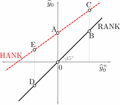
Figure 1. Optimal level of by
0
in HANK (Ω = 0) and RANK absent markup shocks
First, suppose, by
n
0
= 0. In RANK, it is optimal to track this and to set by
0
= by
n
0
= 0. But in HANK there
is a first order benefit from cutting interest rates to reduce inequality, creating a boom in output, until
the marginal benefit of an additional reduction in nominal rates is outweighed by the cost of distorting
output further above its efficient level (point A in Figure 1). Next, suppose that by
n
0
> 0. Again, the
RANK planner sets by
0
= by
n
0
(denoted by point B in the Figure). If the HANK planner were also to set
by
0
= by
n
0
> 0, this would already generate a surprise fall in interest rates, which would reduce inequality to
some extent. The HANK planner still perceives some additional benefit to reducing inequality further but
the marginal benefit is smaller since inequality has already been reduced. Consequently, it is not optimal
to deviate as much from productive efficiency as in the case by
n
0
= 0, and so the gap between points C and
B is smaller than that between points A and the origin. Conversely, when by
n
0
< 0, tracking the flexible
price allocation would entail a surprise interest rate increase which would increase consumption inequality.
The benefit of deviating from this RANK allocation is larger in this case and therefore it is optimal to
tolerate a larger deviation from production efficiency: the gap between points D and E is larger than that
between point A and the origin.
Finally, the date 0 target criterion puts less weight on inflation relative to output α > 1. This is because,
given the constraint on monetary policy imposed by (36), the evolution of consumption inequality depends
directly on the sequences {by
t
, by
n
t
}
∞
t=0
but not on inflation. Thus, the target criterion puts relatively less
weight on inflation and more on output, which attains heightened importance due to its effects on inequality.
Figure 2 shows the dynamics of optimal policy absent shocks in the economy with Ω = 0. The policy
maker cuts nominal interest rates at date 0 (panel d), which generates a fall in real rates and in the
passthrough from income risk to consumption risk µ
t
(panel e). The fall in consumption risk in turn
reduces consumption inequality on impact (panel c), after which it gradually returns to steady state. The
fall in interest rates also generates a boom in output (panel a) and inflation (panel b). Since there are no
shocks to the efficient level of output in this scenario, both the boom in output and increase in inflation
are in themselves undesirable from an efficiency perspective, even if they are a price worth paying for
a persistent reduction in inequality. In order to arrest the increase in inflation, the planner commits to
tighten policy, generating a fall in output and deflation, from date 1 onwards. Since firms are forward
looking, a commitment to lower inflation in the future mitigates the date 0 inflation caused by the boom
20
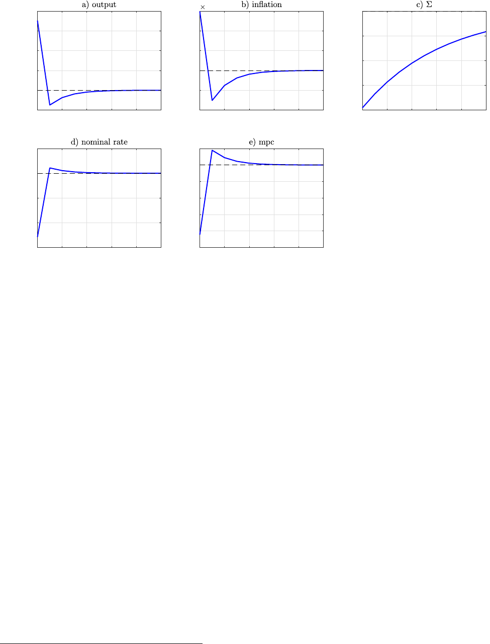
0 2 4 6 8 10
-0.02
0
0.02
0.04
0.06
0.08
0 2 4 6 8 10
-2
-1
0
1
2
3
10
-3
0 2 4 6 8 10
-0.02
-0.015
-0.01
-0.005
0
0 2 4 6 8 10
-0.3
-0.2
-0.1
0
0.1
0 2 4 6 8 10
-0.25
-0.2
-0.15
-0.1
-0.05
0
0.05
Figure 2. Time Inconsistency: Optimal dynamics absent shocks. All variables are plotted as percentage deviations from
their steady state values.
in output.
Next, we discuss the optimal dynamic response of the economy to a negative productivity shock. Figure
3 shows the impulse responses to a negative productivity shock under optimal policy in the HANK and
RANK models, defined as the difference between outcomes with and without the shock. That is, for any
variable of interest x, we plot x
t
|
z
0
=−0.01
−x
t
|
z
0
=0
.
17
In the RANK economy (red lines), the planner allows
output to fall (panel a) in line with the natural rate of output, keeping the output gap (panel f) and
inflation (panel b) equal to zero. Implementing a fall in output requires an increase in nominal interest
rates (panel d), but since agents do not face idiosyncratic risk, this has no effect on consumption inequality
which is always zero.
In the HANK economy (blue lines), a sharp increase in interest rates would increase the passthrough
from income to consumption risk and would persistently increase inequality. To avoid this, the planner
actually cuts interest rates at date 0, dampening the increase in passthrough µ
t
and the increase in
inequality. Output does not fall as much as the flexible price level of output (as shown by the output gap
in panel f), and as a result inflation increases at date 0 - even relative to the scenario absent shocks. This
increase in inflation is not costless. To mitigate its impact, the planner commits to a slightly higher path
of interest rates, and lower output and inflation, from date 1 onwards.
Understanding the forces generating time inconsistency The difference in the optimal target
criterion than at all other dates arises only because there is existing wealth inequality at the start of date
0. Suppose that there is an equalization of asset positions across all households at the beginning of date 0.
17
In the RANK economy, the impulse response is identical to the response of the economy to the shock, since in the absence
of shocks, optimal policy keeps all variables at their steady state values and all deviations from steady state equal zero. This
is not true in the HANK economy, where (as shown in Figure 2) the Ramsey planner deviates from steady state even absent
shocks.
21
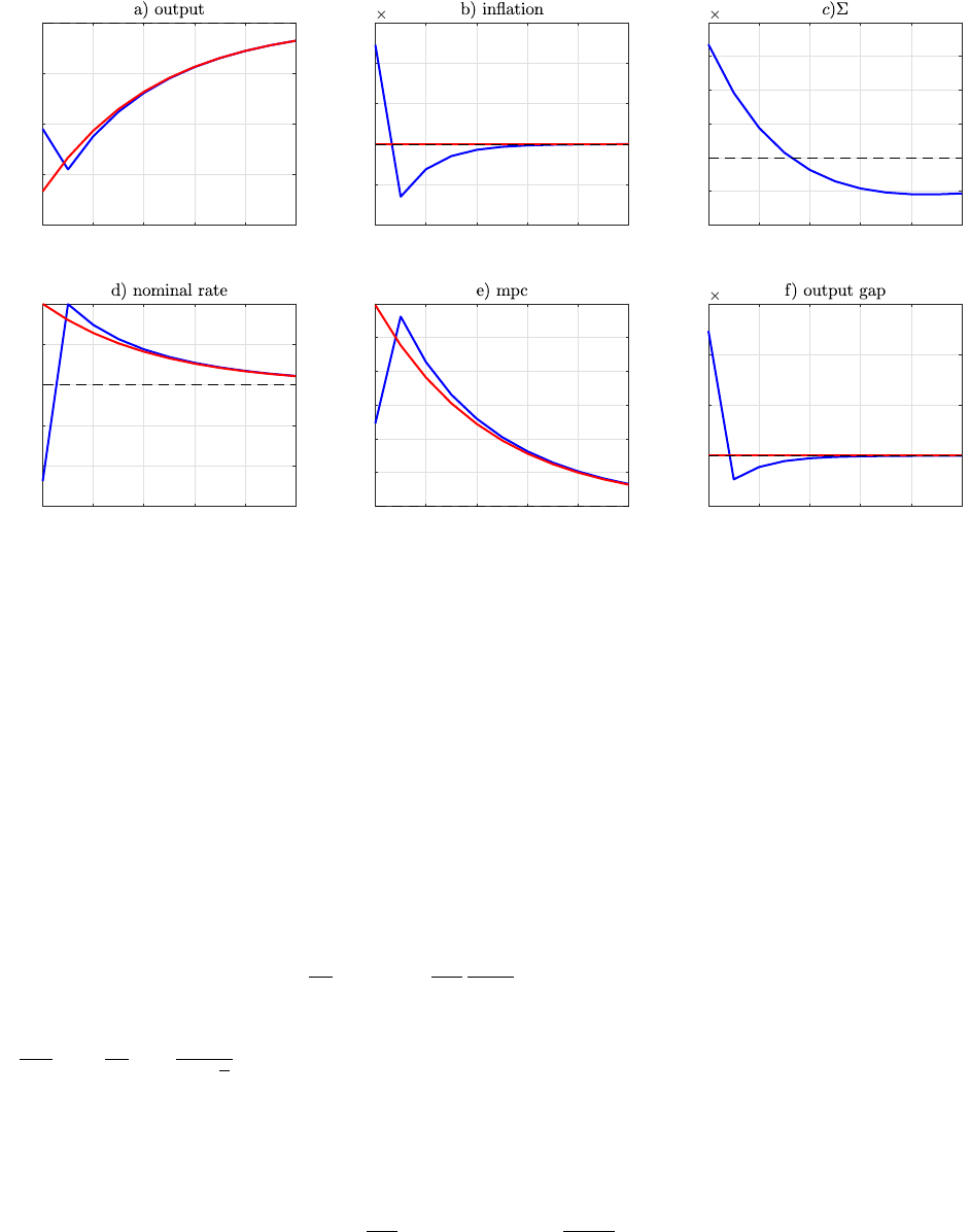
0 2 4 6 8 10
-0.04
-0.03
-0.02
-0.01
0
0 2 4 6 8 10
-4
-2
0
2
4
6
10
-4
0 2 4 6 8 10
-1
-0.5
0
0.5
1
1.5
2
10
-3
0 2 4 6 8 10
-0.03
-0.02
-0.01
0
0.01
0.02
0 2 4 6 8 10
0
0.01
0.02
0.03
0.04
0.05
0.06
0 2 4 6 8 10
-5
0
5
10
15
10
-3
Figure 3. HANK (Ω = 0) vs RANK optimal response to a negative productivity shock. Red line denotes RANK while
blue line represents HANK (Ω = 0). All variables are plotted as percentage deviations from their steady state values. In panel
f), we plot output gap as the difference between y
t
and y
n
t
normalized by steady state y: (by
t
/y) − (by
n
t
/y).
In this scenario, the URE channel is inoperative, as discussed in section 4 and surprise changes in µ
0
have
no additional effect relative to anticipated changes. When there is existing wealth inequality, a surprise cut
in the path of interest rates (lower µ
0
) lowers the consumption of rich savers and raises the consumption
of poor borrowers, reducing consumption inequality. Consequently, at t = 0, the planner deviates from the
date t > 1 target criterion by cutting interest rates do engineer precisely this outcome. Absent existing
wealth inequality at the beginning of date 0, clearly there are no borrowers and savers to redistribute
between and this motive is absent. In fact, with Ω = 0, absent initial wealth inequality, equation (37)
becomes:
b
Σ
t
Σ
= ΛΓ
t
+
ϑ
βR
b
Σ
t−1
Σ
∀t ≥ 0 (43)
with
b
Σ
−1
Σ
= −
βR
ϑ
ln
1−ϑ
1−ϑe
Λ
2
< 0. Equation (43) shows that without initial wealth inequality, the planner
is unable to affect Σ
t
at any date (up to first-order). Unsurprisingly then, the planner faces the standard
trade-off between price stability and productive inefficiency. Consequently, the optimal target criterion at
all dates in this case simplifies to:
(by
t
− by
n
t
) −
1
βR
by
t−1
− by
n
t−1
+
λ
λ − 1
π
t
= 0 (44)
with by
−1
= by
n
−1
= 0 and so divine coincidence holds - optimal policy implements π
t
= 0 and by
t
= by
n
t
at all
dates t ≥ 0 in response to productivity shocks.
Remark 2 (The interest rate exposure channel versus the Fisher channel). Previous research has shown
22

how the redistribution of wealth through inflation when assets and liabilities are nominal may create an
inflationary bias on the part of the central bank. This “Fisher channel” is absent in our baseline economy
where households only hold real assets: the planner is unable to redistribute real wealth via surprise infla-
tion. Nonetheless, the planner can redistribute consumption via a surprise cut in the path of real rates via
the interest rate exposure channel (Auclert, 2019). Auclert (2019) studies how both these channel mediate
the effect of interest rate changes on aggregate consumption in an environment with MPC heterogeneity.
In our economy, all agents have the same MPC, so monetary policy does not affect aggregate consumption
through these channels. However, it does affect the distribution of consumption and in our baseline econ-
omy, optimal monetary policy deliberately utilizes the interest rate exposure channel to reduce consumption
inequality. In Section 6, when we introduce nominal bonds into our model, optimal monetary policy exploits
both channels to achieve the same ends.
5.4.2 Optimal policy with countercyclical risk
While the case with Ω = 0 is a useful benchmark to understand the forces driving optimal monetary policy,
the empirically relevant case is one of countercyclical risk, which implies that Ω > 0.
18
In this case a cut in
interest rates, and the associated boom in output (and wages), reduce consumption risk through both the
income risk and self-insurance channels. With Ω = 0, risk was procyclical, and the benefit of lower interest
rates (which lower µ and increase households’ ability to self insure) was exactly balanced by the cost of
the associated boom in output which increased the level of income risk faced by households. In contrast,
when risk is countercyclical, the increase in output actually reduces the level of income risk, at the same
time as lower interest rates improve households’ ability to self-insure: expansionary policy unambiguously
reduces consumption risk and inequality. This can be seen by substituting (34) into (33):
b
Σ
t
Σ
=
−γ
1 −
e
β
Ωby
t
+ ΛΓ
t
+
ϑ
βR
b
Σ
t−1
Σ
for t > 0
−γ
1 −
e
β
Ωby
0
+ ΛΓ
0
+
ϑΛΣ
1−ϑ
bµ
0
for t = 0
(45)
When Ω > 0, an increase in output by
t
reduces the consumption risk faced by households at any date,
not just at date 0:
∂
b
Σ
t
∂ ˆy
t
< 0. In this environment, the planner would only refrain from increasing output
if doing so distorts productive efficiency and creates inflation. Indeed recall from (26) that in steady state
with Ω > 0, the marginal benefit of reducing inequality by stimulating demand is exactly balanced by
the cost of deviating further from production inefficiency. The reason a marginal increase in output has a
first-order cost in terms of productive efficiency is that the steady state in this case features an inefficiently
high level of output y > 1 (also reflected in w > 1). Out of steady state the planner faces a similar trade-off
between the benefit of reducing inequality via higher output and the cost of further distorting productive
efficiency, while also seeking to limit deviations from price stability. This tradeoff informs the optimal
design of monetary policy, as we discuss next.
18
More precisely, countercyclical risk (Θ > 1) implies Ω >
Λ
(1−
e
β)(1−Λ)
> 0. When 0 < Ω <
Λ
(1−
e
β)(1−Λ)
, risk is weakly
procyclical so expansionary monetary policy reduces pass through than it increase income risk, reducing consumption risk in
net.
23

Proposition 4 (Optimal monetary policy with countercyclical risk). Output and inflation {by
t
, π
t
}
∞
t=0
under optimal policy satisfy
η
t
=
α
0
(Ω)
by
t
− δ
0
(Ω)by
n
t
− χ(Ω)
for t = 0
α(Ω)
by
t
− δ(Ω)by
n
t
for t ≥ 1
(46)
η
t
=
1
βR
η
t−1
−
λ
λ − 1
yπ
t
(47)
π
t
=
e
β
ϑ
π
t+1
+ κ(by
t
− by
e
t
) + u
t
(48)
where α(Ω), δ(Ω), α
0
(Ω), δ
0
(Ω) and χ(Ω) are defined in Appendix E.1 and satisfy α
0
(0) = α, δ
0
(0) = δ,
χ(0) = χ, α(0) = 1, δ(0) = 1. Further, when risk is countercyclical α(Ω), α
0
(Ω) > 1 and δ(Ω), δ
0
(Ω) < 1.
Proof. See Appendix E.1.
By combining (46) with (48), one can derive the optimal target criterion for t = 0:
by
0
− δ
0
(Ω)by
n
0
+
λ
λ − 1
y
α
0
(Ω)
π
0
= χ(Ω) for t = 0 (49)
and for dates t > 1:
by
t
− by
t−1
− δ(Ω)
by
e
t
− by
∗
t−1
+
λ
λ − 1
y
α(Ω)
π
t
= 0 (50)
As in the case Ω = 0, optimal policy deviates from RANK at date 0, creating a boom even absent
exogenous shocks. However, unlike in the case Ω = 0, with countercyclical risk optimal policy also deviates
from the RANK target criterion at subsequent dates t > 1. This should not be not surprising: with Ω = 0,
monetary policy can only affect the evolution of consumption inequality (to first order) at date 0. However,
with countercyclical risk, an expansion in output reduces inequality at all dates, so monetary policy faces
a tradeoff between the benefits of lower inequality and the cost of distorting productive efficiency and
price stability at all dates, and deviates from RANK as a result. In particular, δ(Ω) < 1 when risk is
countercyclical: output tracks the flexible price level of output less than one for one at all dates. In
addition, α(Ω) > 1: the planner puts more weight on stabilizing output relative to inflation at all dates.
To understand why output moves less than one-for-one with its flexible price level at all date, δ(Ω) < 1,
recall the distinction between three different levels of output: the productively efficient level of output y
e
t
,
the flexible price level of output y
n
t
, and the equilibrium level of output y
t
. When Ω = 0, y
n
t
= y
e
t
. In
this case, the standard subsidy corrects for the distortion due to monopolistic competition, and productive
efficiency is obtained when there is zero inflation at all dates, or when prices are flexible. In other words, the
flexible price version of the economy with Ω = 0 features a zero labor wedge at all dates, T
t
≡ ln z
t
−ln w
n
t
= 0
where w
n
t
denotes the wage consistent with the flexible price level of output.
However, with countercyclical risk, Ω > 0, and the flexible price level of output y
n
t
is higher than the
efficient level of output y
e
t
, whatever the level of productivity. In this case, firms enjoy a subsidy which is
larger than the one necessary to eliminate the distortion due to monopolistic competition (see eq. (27)), and
output would be inefficiently high under flexible prices. The flexible price version of this economy features
a negative labor wedge - a net subsidy to output and employment - at all times. Consequently keeping
24
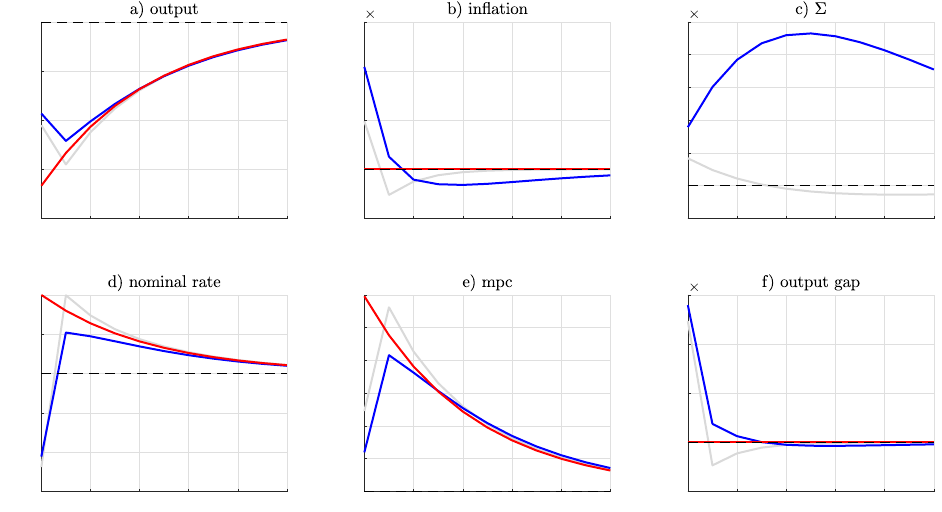
z
0 2 4 6 8 10
-0.04
-0.03
-0.02
-0.01
0
0 2 4 6 8 10
-5
0
5
10
15
10
-4
0 2 4 6 8 10
-2
0
2
4
6
8
10
10
-3
0 2 4 6 8 10
-0.03
-0.02
-0.01
0
0.01
0.02
0 2 4 6 8 10
0
0.01
0.02
0.03
0.04
0.05
0.06
0 2 4 6 8 10
-5
0
5
10
15
10
-3
Figure 4. HANK (Ω > 0) vs RANK optimal response to a negative productivity shock. Red line denotes RANK, blue
line represents HANK with countercyclical risk (Ω > 0), and gray line represents HANK with Ω = 0. All variables are plotted
as percentage deviations from their steady state values. In panel f), we plot output gap as the difference between y
t
and y
n
t
normalized by steady state y: (by
t
/y) − (by
n
t
/y).
output equal to its flexible price level entails keeping output inefficiently high at all times. Conversely,
in order to set output equal to its efficient level, and undo the effects of the net subsidy to output and
employment, one would have to drive output y
t
down below its flexible price level y
n
t
.
Absent shocks, the planner could always implement the efficient level of output by raising interest
rates above their steady state level, reducing output below its inefficiently high flexible price level, and
eliminating the negative labor wedge. She chooses not to do this, however, because the cost in terms of
increased consumption inequality is too high - so she sets output equal to its flexible price level.
Now consider a scenario in which productivity is higher than in steady state (z > 1). In this case, the
planner could continue to set output equal to its flexible price level, keeping the labor wedge unchanged
(T
t
= ln z
t
− ln w
t
= −ln w < 0). This would entail increasing y
t
one for one with y
n
t
. But it is no
longer optimal to do so. The only reason the planner does not eliminate the inefficient subsidy in steady
state is that doing so would increase inequality too much. Now however, with higher output, consumption
inequality is already lower, and the benefit of the inefficient subsidy is lower: even if the planner were
to implement a lower level of output relative to the flexible price level, improving productive efficiency,
inequality would still be relatively low. Optimal policy seeks to reduce the magnitude of the labor wedge
by bringing the level of output y
t
closer to the efficient level of output y
e
t
. Since 1 = y
e
< y
n
= y in steady
state, this entails by
t
< by
n
t
.
Conversely, suppose productivity falls relative to steady state, z < 1. Again, the planner could track
the flexible price level of output y
n
t
, keeping the labor wedge unchanged. Doing so would entail reducing
output one for one with the flexible price level of output. But when output is lower, consumption inequality
is higher. In this case, the rationale for keeping output above its efficient level y
e
t
is not eliminated - it
25
is actually strengthened. It is optimal to deviate even further from productive efficiency, increase the
effective subsidy to output and employment, and reduce output less than one for one with the efficient
level of output.
Figure 4 shows the impulse responses to a negative productivity shock under optimal policy in HANK
with countercyclical risk (blue lines), with outcomes in RANK (red lines) and HANK with Ω = 0 (gray
lines) shown as benchmarks. As in the benchmark with Ω = 0, the planner deviates from optimal policy in
RANK - which tracks the flexible price level of output - by cutting nominal interest rates at date 0 (panel
d) and mitigating the fall in output (panel a) on impact, at the cost of creating an increase in inflation
(panel b). Recall that in the economy with Ω = 0, the planner attempted to dampen this increase in
inflation by committing to tighter policy starting at date 1. With countercyclical risk, however, any fall
in output is costly because it directly increases inequality. Indeed, even under optimal policy, the path of
inequality is higher with countercyclical risk (panel c). To prevent inequality from rising even more, the
planner postpones the commitment to tighter policy in the future. While interest rates still rise at date 1
(blue line in panel d), the increase is smaller than in the RANK economy (red line) or the HANK economy
with Ω = 0 (gray line). As a result, the fall in inflation and output-gap are also smoothed out over time.
Remark 3 (The role of initial wealth inequality with countercyclical risk). With countercyclical risk
(Ω > 0), the optimal target criterion is different at date t = 0 and at all subsequent dates, as was the case
when Ω = 0. In particular, optimal policy features a boom at date 0 even absent exogenous shocks. As in
the Ω = 0 case, such a policy is optimal because given existing wealth inequality at date 0, a surprise cut
in interest rates raises the consumption of poor borrowers and reduces the consumption of rich savers. To
understand the role of wealth inequality in driving this result, suppose again that there is an equalization
of household wealth at the beginning of date 0. In this case, the optimal target criterion (50) characterizes
optimal policy at all dates (with by
−1
= by
∗
−1
= 0). This implies that absent shocks, the planner keeps interest
rates at their steady state value. However, unlike in the case with Ω = 0 and wealth equalization, it is no
longer optimal to implement zero inflation and replicate flexible price allocations in response to productivity
shocks - even though it remains feasible to do so.
Figure 5 plots dynamics under optimal policy in this scenario. Qualitatively, policy is similar to the
case without wealth equalization in which there is a time inconsistency problem. Relative to RANK, the
planner implements a lower increase in interest rates on impact (panel d), resulting in a lower increase
in output (panel a) and the passthrough from income to consumption risk µ
t
(panel e). This comes at the
cost of a short-lived increase in inflation. Note that inequality (shown in the panel c) is below its steady
state level, despite the increase in income risk caused by the fall in output, because the initial equalization
of wealth reduces consumption inequality at the start of date 0.
6 Nominal debt
So far we have considered an economy in which households traded inflation indexed bonds. As mentioned
in Remark 2, we made this assumption to distinguish between two ways in which monetary policy can
affect the distribution of consumption in HANK economies. The first is the interest rate exposure channel:
an unanticipated fall in real interest rates increases the consumption of poor debtors and reduces that of
rich savers. The second is the Fisher effect: unanticipated inflation redistributes real wealth from savers
26
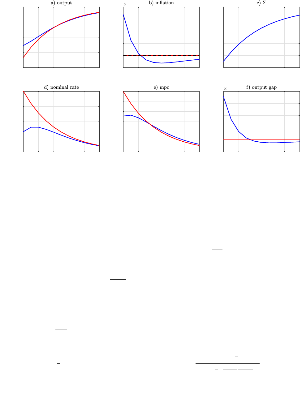
0 2 4 6 8 10
-0.04
-0.03
-0.02
-0.01
0
0 2 4 6 8 10
-2
0
2
4
6
8
10
-4
0 2 4 6 8 10
-0.1
-0.08
-0.06
-0.04
-0.02
0
0 2 4 6 8 10
0
0.005
0.01
0.015
0.02
0 2 4 6 8 10
0
0.01
0.02
0.03
0.04
0.05
0.06
0 2 4 6 8 10
-2
0
2
4
6
8
10
-3
Figure 5. HANK (Ω > 0) vs RANK optimal response to a negative productivity shock in the economy with wealth
equalization at the beginning of date 0. Red line denotes RANK, blue line represents HANK with countercyclical risk (Ω > 0).
All variables are plotted as percentage deviations from their steady state values. In panel f), we plot output gap as the
difference between y
t
and y
n
t
normalized by steady state y: (by
t
/y) − (by
n
t
/y).
who hold nominal assets to debtors with nominal liabilities. Our baseline model with inflation indexed
debt abstracts altogether from the second effect to focus on the first. In this section, we allow households
to trade nominal debt and show how the the presence of the Fisher effect changes the optimal conduct of
monetary policy.
Financial intermediaries now trade nominal claims at nominal price
ϑ
1+i
t
which pay a dollar tomorrow.
Then the household’s budget constraint can be written as:
P
t
c
s
t
(i) +
ϑ
1 + i
t
A
s
t+1
(i) = P
t
w
t
`
s
t
(i) + A
s
t
(i) + P
t
T
t
where A
s
t+1
(i) is the quantity of nominal claims purchased by the household at date t. The details of this
extension are in Appendix F. As before the evolution of this economy is characterized by the aggregate IS
equation (11), the evolution of µ(12), Phillips curve (7), the definition of GDP (15) and the evolution of
Σ, replacing R
t
=
1+i
t
Π
t+1
. Four of these five equations are unaffected by the introduction of nominal bonds
- the exception is the evolution of Σ, which becomes:
19
ln Σ
t
=
1
2
γ
2
µ
2
t
w
2
t
σ
2
t
+ ln [1 − ϑ + ϑΣ
t−1
] + I(t = 0) ln
1 − ϑe
Λ
2
1 − ϑe
Λ
2
µ
0
E
−1
µ
0
E
−1
Π
0
Π
0
2
(51)
(51) shows that the presence of nominal debt means that unanticipated higher inflation reduces consump-
tion inequality. Since there are no aggregate shocks except at date 0 and the Ramsey planner can only
re-optimize at date 0, actual and expected inflation coincide in equilibrium except at date 0. As Appendix
19
See Appendix F for the derivation.
27
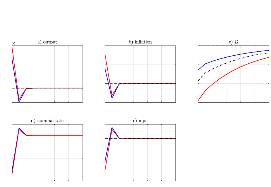
F details, the cohort born at date s < 0 enters date 0 with with a cross-sectional distribution of real
wealth which is N
0, −sw
2
σ
2
E
−1
Π
0
Π
0
2
. Higher than expected inflation Π
0
> E
−1
Π
0
compresses the
distribution of real wealth. Thus, by generating inflation at date 0, the planner can reduce wealth and
hence consumption inequality. This reduction in consumption inequality is in addition to the reduction
achieved by the surprise cut in interest rates at date 0.
0 2 4 6 8 10
-5
0
5
10
15
10
-3
0 2 4 6 8 10
-0.02
-0.01
0
0.01
0.02
0.03
0.04
0 2 4 6 8 10
-0.015
-0.01
-0.005
0
0 2 4 6 8 10
-0.08
-0.06
-0.04
-0.02
0
0.02
0 2 4 6 8 10
-0.06
-0.04
-0.02
0
0.02
Figure 6. Time inconsistency with nominal debt: Optimal dynamics absent shocks in alternative calibration (κ = 0.5).
Blue line denotes HANK with countercylcical risk and real debt, red line denotes HANK with countercyclical risk and nominal
debt. All variables are plotted as percentage deviations from their steady state values.
Qualitatively, this increases the planner’s incentive to create a boom at date 0 even absent aggregate
shocks. Quantitatively, though, this effect is small in our baseline calibration, as Figure 8 in Appendix
F shows - optimal policy in the two economies is essentially identical. This is primarily because in our
baseline calibration, the Phillips curve is relatively flat (κ = 0.01) which means that even a large cut in
real interest rates, and a large boom in output, generates only a small increase in inflation. In order to
generate a large enough increase in inflation to effect significant redistribution, it would be necessary to
engineer a massive deviation from the productively efficient level of output, and it is not optimal for the
planner to do this.
To illustrate the qualitative effect of introducing inflation-indexed debt, Figure 6 shows optimal policy
absent shocks with a steeper Phillips curve (κ = 0.5). As panel b shows, the planner creates a larger increase
in inflation in the economy with nominal debt (red line) than in the economy with inflation-indexed debt
(blue line). This results in a larger reduction in inequality (panel c). The black dashed line in this panel
shows the effect of implementing the optimal policy from the economy with inflation-indexed debt in the
economy with nominal debt. Even if the planner follows this policy, and does not actively exploit the
Fisher effect, this already automatically generates a larger reduction in inequality than in the economy
with inflation-indexed debt (the black dashed line is below the blue line) because the same increase in
inflation now redistributes real wealth. The planner actually generates a further increase in inflation, and
28
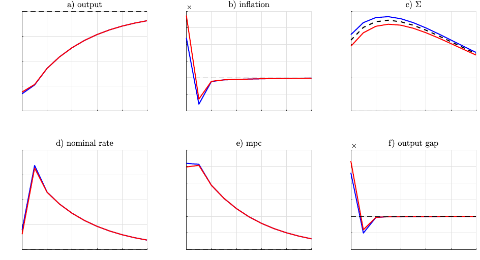
0 2 4 6 8 10
-0.04
-0.03
-0.02
-0.01
0
0 2 4 6 8 10
-4
-2
0
2
4
6
8
10
-3
0 2 4 6 8 10
0
0.005
0.01
0.015
0 2 4 6 8 10
0
0.005
0.01
0.015
0.02
0 2 4 6 8 10
0
0.01
0.02
0.03
0.04
0.05
0.06
0 2 4 6 8 10
-2
-1
0
1
2
3
4
10
-3
Figure 7. Nominal vs inflation indexed debt: optimal response to a negative productivity shock in alternative calibration
(κ = 0.5). Blue line represents HANK with countercyclical risk and real debt, red line denotes HANK with countercyclical
risk and nominal debt. All variables are plotted as percentage deviations from their steady state values. In panel f), we plot
output gap as the difference between y
t
and y
n
t
normalized by steady state y: (by
t
/y) − (by
n
t
/y).
so inequality falls even more (the red line is below the black dashed line).
The presence of nominal assets and liabilities also affects the optimal response to shocks. Figure 7 plots
the impulse responses (defined as in the previous section) to a negative productivity shock under optimal
policy in the alternative calibration with κ = 0.5. Allocations under optimal policy in the economy with
nominal debt (red line) are similar to those with inflation-indexed debt (blue line), even with a steep
Phillips curve. However, the level of output now deviates even more from y
n
t
(panel f) in order to generate
a larger surprise increase in inflation (panel b). This is optimal when risk is countercyclical because negative
productivity shock tends to increase inequality (panel c). Creating more surprise inflation partially offsets
this, yielding a lower increase in inequality (red line) than would obtain if the planner followed the same
policy as in the economy with inflation-indexed debt (black dashed line). As in the previous figure, though,
even following this same policy would automatically generate a larger reduction in inequality than in the
economy with inflation-indexed debt (blue line).
7 Conclusion
We use a analytically tractable HANK model to study how monetary policy affects inequality, and the
extent to which this warrants a change in the principles governing the design of monetary policy which have
been developed in the Representative Agent New Keynesian literature. In a complete markets economy,
monetary policy affects output and inflation but, trivially, has no effects on inequality (since households
can use Arrow securities to insure themselves, eliminating consumption inequality). In our incomplete
markets economy, monetary policy affects consumption risk and inequality through four channels. The
29

first is the income risk channel: when the idiosyncratic income risk faced by households is countercyclical,
expansionary monetary policy, by generating a boom in output, tends to reduce income risk and inequality.
More subtly, lower interest rates make it easier for households to self-insure against income shocks, reducing
consumption risk for a given level of income risk - the self-insurance channel. Finally, unexpected cuts in
interest rates redistribute consumption through an unhedged interest rate exposure channel, and unexpected
inflation redistributed real wealth through the Fisher channel. Thus, expansionary monetary policy can
reduce consumption inequality through all four of these channels.
Given that monetary policy has this power to reduce inequality, how and when should it be used? A
utilitarian planner trades off the benefits of lower inequality against the costs of pushing up output and
inflation above their efficient levels. In recessions, inequality is already high - in the relevant case with
countercyclical risk - so the marginal benefit of reducing inequality is particularly high. Consequently,
optimal monetary policy is more accommodative in recessions relative in to a RANK benchmark: the
planner prevents output from falling as much as the efficient level of output, even though this entails
higher inflation, because curtailing the fall in output also curtails the rise in inequality.
References
Acharya, Sushant and Keshav Dogra, “Understanding HANK: insights from a PRANK,” Staff Reports
835, Federal Reserve Bank of New York February 2018.
Angeletos, George-Marios and Laurent Emmanuel Calvet, “Idiosyncratic Production Risk, Growth
and the Business Cycle,” Journal of Monetary Economics, 2006, 53, 1095 – 1115.
Auclert, Adrien, “Monetary Policy and the Redistribution Channel,” American Economic Review, 2019,
109 (6), 2333 – 2367.
, Matt Rognlie, and Ludwig Straub, “The Intertemporal Keynesian Cross,” Working Paper 25020
2018.
Bhandari, Anmol, David Evans, Mikhail Golosov, and Thomas J Sargent, “Inequality, Business
Cycles and Monetary-Fiscal- Policy,” Working Paper 24710, National Bureau of Economic Research
June 2018.
Bilbiie, Florin O., “Limited Asset Markets Participation, Monetary Policy and (Inverted) Aggregate
Demand Logic,” Journal of Economic Theory, May 2008, 140 (1), 162–196.
, “Monetary Policy and Heterogeneity: An Analytical Framework,” Working Paper, November 2019.
, “The New Keynesian Cross: Understanding Monetary Policy with Hand-to-Mouth Households,” Jour-
nal of Monetary Economics, 2019, Forthcoming.
and Xavier Ragot, “Optimal Monetary Policy and Liquidity with Heterogeneous Households,” Work-
ing Papers 2018.
Blanchard, Olivier Jean and Jordi Gal´ı, “Real Wage Rigidities and the New Keynesian Model,”
Journal of Money, Credit and Banking, 2007, 39, 35 – 65.
30

Caballero, Ricardo J., “Consumption Puzzles and Precautionary Savings,” Journal of Monetary Eco-
nomics, 1990, 25 (1), 113 – 136.
Cagetti, Marco, “Wealth Accumulation over the Life Cycle and Precautionary Savings,” Journal of
Business & Economic Statistics, 2003, 21 (3), 339–353.
Calvet, Laurent Emmanuel, “Incomplete Markets and Volatility,” Journal of Economic Theory, 2001,
98, 295 – 338.
Calvo, Guillermo A and Maurice Obstfeld, “Optimal Time-Consistent Fiscal Policy with Finite
Lifetimes,” Econometrica, 1988, 56 (2), 411–432.
Challe, Edouard, “Uninsured Unemployment Risk and Optimal Monetary Policy in a Zero-Liquidity
Economy,” American Economic Journal: Macroeconomics, April 2020.
Christelis, Dimitris, Dimitris Georgarakos, Tullio Jappelli, and Maarten van Rooij, “Con-
sumption Uncertainty and Precautionary Saving,” CSEF Working Papers 421, Centre for Studies in
Economics and Finance (CSEF), University of Naples, Italy December 2015.
Cui, Wei and Vincent Sterk, “Quantitative Easing,” Working Papers, UCL 2019.
Debortoli, Davide and Jordi Gal´ı, “Monetary Policy with Heterogeneous Agents: Insights from TANK
models,” Working Paper 2018.
den Haan, Wouter, Pontus Rendahl, and Markus Riegler, “Unemployment (Fears) and Deflation-
ary Spirals,” Journal of the European Economic Assocation, 2018, 16(5), 1281 – 1349.
Fagereng, Andreas, Luigi Guiso, and Luigi Pistaferri, “Firm-Related Risk and Precautionary Saving
Response,” American Economic Review, May 2017, 107 (5), 393–97.
Gal´ı, Jordi, Monetary Policy, Inflation, and the Business Cycle: An Introduction to the New Keynesian
Framework and Its Applications, Second Edition, Princeton University Press, 2015.
Gal´ı, Jordi, David Lopez-Salido, and Javier Valles, “Understanding the Effects of Government
Spending on Consumption,” Journal of the European Economic Association, 2007, 5 (1), 227–270.
Guvenen, Fatih, Serdar Ozkan, and Jae Song, “The Nature of Countercyclical Income Risk,” Journal
of Political Economy, 2014, 122 (3), 621–660.
Kaplan, Greg, Benjamin Moll, and Giovanni L. Violante, “Monetary Policy According to HANK,”
American Economic Review, March 2018, 108 (3), 697–743.
Kekre, Rohan, “Unemployment Insurance in Macroeconomic Stabilization,” Working Paper 2019.
McKay, Alisdair and Ricardo Reis, “The Role of Automatic Stabilizers in the U.S. Business Cycle,”
Econometrica, January 2016, 84, 141–194.
and , “Optimal Automatic Stabilizers,” Working Paper 2019.
31

, Emi Nakamura, and Jon Steinsson, “The Power of Forward Guidance Revisited,” American
Economic Review, October 2016, 106 (10), 3133.
Nistic`o, Salvatore, “Optimal Monetary Policy And Financial Stability In A Non-Ricardian Economy,”
Journal of the European Economic Association, October 2016, 14 (5), 1225–1252.
Nu˜no, Galo and Carlos Thomas, “Optimal Monetary Policy with Heterogeneous Agents,” Working
Papers 1624, Banco de Espana November 2019.
Ravn, Morten O. and Vincent Sterk, “Job Uncertainty and Deep Recessions,” Journal of Monetary
Economics, 2017, 90 (C), 125–141.
and , “Macroeconomic Fluctuations with HANK & SAM: An Analytical Approach,” Journal of the
European Economic Association, Forthcoming.
Rotemberg, Julio J., “Monopolistic Price Adjustment and Aggregate Output,” Review of Economic
Studies, 1982, 49 (4), 517–531.
Wang, Neng, “Caballero Meets Bewley: The Permanent-Income Hypothesis in General Equilibrium,”
American Economic Review, June 2003, 93 (3), 927–936.
Werning, Ivan, “Incomplete Markets and Aggregate Demand,” Working Paper 21448, National Bureau
of Economic Research August 2015.
32

Appendix
A Proof of Proposition 1
The date s problem of an individual i born at date s can be written as:
max
{c
s
t
(i),`
s
t
(i),b
s
t+1
(i)}
−
∞
X
t=s
(βϑ)
t−s
1
γ
e
−γc
s
t
(i)
+ ρe
1
ρ
[`
s
t
(i)−ξ
s
t
(i)]
s.t.
c
s
t
(i) + q
t
b
s
t+1
(i) = w
t
`
s
t
(i) + b
s
t
(i) + T
t
(52)
where b
s
s
(i) = 0 and w
t
= (1 − τ) ew
t
. The optimal labor supply decisions of houshold i is given by:
`
s
t
(i) = ρ ln w
t
− ργc
s
t
(i) + ξ
s
t
(i) (53)
and the Euler equation is given by:
e
−γc
s
t
(i)
= βR
t
E
t
e
−γc
s
t+1
(i)
(54)
where we have used the fact that q
t
=
ϑ
R
t
. Next, guess that the consumption decision rule takes the form:
c
s
t
(i) = C
t
+µ
t
x
s
t
(i) (55)
where x
s
t
(i) = b
s
t−1
(i) + w
t
ξ
s
t
(i) − ξ
denotes “virtual cash-on-hand”. Notice that x
s
t+1
(i) is normally
distributed and so given the guess (55), c
s
t+1
(i) is also normally distributed with mean:
E
t
c
s
t+1
(i) = C
t+1
+ µ
t+1
R
t
ϑ
x
s
t
(i) + w
t
ρ ln w
t
+
¯
ξ
+ T
t
− (1 + ργw
t
) c
s
t
(i)
and variance:
V
t
c
s
t+1
(i)
= µ
2
t+1
w
2
t+1
σ
2
t+1
Taking logs of (54) and using the two expressions above:
c
s
t
(i) = −
1
γ
ln βR
t
−
1
γ
ln E
t
e
−γc
s
t+1
(i)
= −
1
γ
ln βR
t
+ E
t
c
s
t+1
(i) −
γ
2
V
t
c
s
t+1
(i)
= −
1
γ
ln βR
t
+ C
t+1
+ µ
t+1
R
t
ϑ
x
s
t
(i) + w
t
ρ ln w
t
+
¯
ξ
+ T
t
− (1 + ργw
t
) c
s
t
(i)
−
γµ
2
t+1
w
2
t+1
σ
2
t+1
2
1

Combining the c
s
t
(i) terms and using (55), the above can be rewritten as:
µ
t+1
R
t
ϑ
(1 + ργw
t
) +
ϑ
R
t
µ
−1
t+1
{C
t
+µ
t
x
s
t
(i)} = −
1
γ
ln βR
t
+ C
t+1
+ µ
t+1
R
t
ϑ
x
s
t
(i) + w
t
ρ ln w
t
+
¯
ξ
+ T
t
−
γµ
2
t+1
w
2
t+1
σ
2
t+1
2
(56)
Matching coefficients:
C
t
= −
ϑµ
t
µ
t+1
R
t
1
γ
ln βR
t
+
ϑµ
t
µ
t+1
R
t
C
t+1
+ µ
t
w
t
ρ ln w
t
+
¯
ξ
+ T
t
−
ϑ
R
t
µ
t
µ
t+1
γµ
2
t+1
w
2
t+1
σ
2
t+1
2
(57)
µ
−1
t
= (1 + ργw
t
) +
ϑ
R
t
µ
−1
t+1
(58)
Notice that (58) is the same as (12) in the main text. Next, in equilibrium, aggregate hours worked is
given by:
`
t
= ρ ln w
t
− γρC
t
+ ξ
and hence aggregate income is:
y
t
= w
t
`
t
+ T
t
= w
t
ρ ln w
t
− γρw
t
C
t
+ w
t
ξ + T
t
Using this in (57) and the fact that C
t
= y
t
yields equation (11) in the main text.
B Planner’s Objective function
B.1 Consumption is normally distributed within cohort
Given the consumption function (9) and the normality of shocks, to consumption of newly born in-
dividuals at any date s is normally distributed with mean y
s
and variance σ
2
c
(s, s) = µ
2
s
w
2
s
σ
2
s
since
they all have zero wealth. Given the linearity of the budget constraint, it follows that newly born
agents’ savings decisions a
s
s+1
(i) are also normally distributed with mean 0 and variance σ
2
a
(s + 1, s) =
R
s
θ
2
[1 − (1 + γρw
s
) µ
s
]
2
w
2
s
σ
2
s
. By induction, it follows that for any cohort born at date s, the cross-
sectional distribution of consumption at any date t > s is normal with mean y
t
and variance
σ
2
c
(t, s) = µ
2
t
σ
2
a
(t, s) + µ
2
t
w
2
t
σ
2
t
(59)
while the distribution of asset holdings is normal with mean 0 and variance
σ
2
a
(t, s) =
R
2
t−1
θ
2
[1 − (1 + γρw
t−1
) µ
t−1
]
2
σ
2
a
(t − 1, s) + w
2
t−1
σ
2
t−1
(60)
2

B.2 Objective function of planner
Substituting labor supply (10) into the objective function, we can write the date 0 expected utility of
individual i from the cohort born at date s going forwards as:
W
s
0
(i) = −
1
γ
E
0
∞
X
t=0
(βϑ)
t
(1 + γρw
t
) e
−γc
s
t
(i)
= −
1
γ
E
0
∞
X
t=0
(βϑ)
t
(1 + γρw
t
) e
−γy
t
−γµ
t
x
s
t
(i)
where we have used labor supply (10), consumption function (9) and the fact that in equilibrium C
t
= y
t
.
We assume that the planner puts a weight of 1 on every individual alive at date 0 and (βϑ)
t
on individuals’
lifetime welfare who will be born at date t > 0. Then the social welfare function can be written as:
W
0
= (1 − ϑ)
0
X
s=−∞
ϑ
−s
Z
W
s
0
(i)di
| {z }
welfare of those alive at date 0
+
∞
X
s=1
(1 − ϑ)β
s
Z
W
s
s
(i)di
| {z }
welfare of the unborn at date 0
Using the definition of W
s
0
(i) and W
s
s
(i), notice that W
0
can be written as:
W
0
= −
1
γ
∞
X
t=0
β
t
(1 + γρw
t
) e
−γy
t
Σ
t
where Σ
t
is defined as:
Σ
t
= (1 − ϑ)
t
X
s=−∞
ϑ
t−s
Z
e
−γµ
t
x
s
t
(i)
di (61)
Thus, we can write W
0
as:
W
0
=
∞
X
t=0
β
t
U
t
where U
t
= −
1
γ
(1 + γρw
t
)e
−γy
t
Σ
t
B.2.1 Derivation of Σ
t
recursion
Write (61) as:
Σ
t
= (1 − ϑ)
Z
e
−γµ
t
x
t
t
(i)
di + (1 − ϑ)
t−1
X
s=−∞
ϑ
t−s
Z
e
−γµ
t
x
s
t
(i)
di
= (1 − ϑ) e
γ
2
µ
2
t
w
2
t
σ
2
t
2
+ (1 − ϑ)
t−1
X
s=−∞
ϑ
t−s
Z
e
−γµ
t
{
a
s
t
(i)+w
t
(
ξ
s
t
(i)−ξ
)}
di
= (1 − ϑ) e
γ
2
µ
2
t
w
2
t
σ
2
t
2
+ (1 − ϑ)
t−1
X
s=−∞
ϑ
t−s
Z
e
−γµ
t
a
s
t
(i)
di
Z
e
−γµ
t
w
t
(
ξ
s
t
(i)−ξ
)
di
= e
γ
2
µ
2
t
w
2
t
σ
2
t
2
"
(1 − ϑ) + (1 −ϑ) ϑ
t−1
X
s=−∞
ϑ
t−1−s
Z
e
−γµ
t
R
t−1
θ
[
µ
−1
t−1
−(1+γρw
t−1
)
]
µ
t−1
x
s
t−1
(i)
di
#
where we have used the fact that a
s
t
(i) =
R
t−1
θ
[1 − (1 + γρw
t−1
) µ
t−1
] x
s
t−1
(i). Also, at all dates t > 0,
3

we know that µ
−1
t−1
− (1 + γρw
t−1
) =
θ
R
t−1
µ
−1
t
. Using this, we have for all t > 0:
ln Σ
t
=
γ
2
µ
2
t
w
2
t
σ
2
t
2
+ ln (1 − ϑ + ϑΣ
t−1
) (62)
which is the same as (22) in the main text. Next, imposing steady state up till date 0, we know that
µ
−1
− (1 + γρw) =
e
β (µ
e
0
)
−1
where µ
e
0
denotes the date −1 expectation of µ
0
. Then we can write Σ
0
as:
Σ
0
= e
γ
2
µ
2
0
w
2
0
σ
2
0
2
"
(1 − ϑ) + (1 −ϑ) ϑ
−1
X
s=−∞
ϑ
−1−s
Z
e
−γ
µ
0
µ
e
0
µx
s
−1
(i)
di
#
(63)
and the variance of consumption for cohorts born at date s < 0 is γ
2
µ
2
σ
2
x
(−1, s) = −sΛ. Therefore:
Σ
0
= e
γ
2
µ
2
0
w
2
0
σ
2
0
2
1 − ϑ
1 − ϑe
Λ
2
µ
0
µ
e
0
2
We also know that in steady state (Σ
−1
= Σ) , [1 − ϑ + ϑΣ
−1
]
1 − ϑe
Λ
2
= (1 −ϑ). Plugging this in the
previous expression yields (23) in the main text:
ln Σ
0
=
γ
2
µ
2
0
w
2
0
σ
2
0
2
+ ln [1 − ϑ + ϑΣ
−1
] + ln
1 − ϑe
Λ
2
1 − ϑe
Λ
2
µ
0
µ
e
0
2
C Some auxiliary results
In the proofs that follow, we shall make liberal use of the following assumptions and results.
Assumption 1. Throughout the paper, we shall assume that:
1. ϑ ≥
1
2
2. βϑ > e
−
1
2
= 0.61
3. σ
2
< σ =
2ρ
2
ln ϑ
−1
γρ
1+γρ
2
2
(
1−
φ
γ
)
ln ϑ
−1
1+2 ln ϑ
+(1−β)
!
2
Lemma 2. Given that βϑ > e
−
1
2
, we have Λ < 1 and
e
β < 1.
Proof. Recall that in steady state, Λ = γ
2
µ
2
w
2
σ
2
> 0, i.e.:
Λ =
σ
2
ρ
2
γρw
1 + γρw
2
1 − βθe
Λ
2
2
Rearranging:
f (Λ) ≡
Λ
1 − βθe
Λ
2
2
=
σ
2
ρ
2
γρw
1 + γρw
2
(64)
4

Now, f (Λ) is increasing for Λ < Λ
∗
≡ −2 ln βϑ < 1 given our assumption, and goes to ∞ as Λ → Λ
∗
. For
any values of σ and ρ, we can find some 0 < Λ < Λ
∗
satisfying f
Λ
=
σ
2
ρ
2
. Thus, any solution to (64)
must satisfy Λ ≤ Λ < Λ
∗
< 1. By construction, for any Λ < Λ
∗
,
e
β = βθe
Λ
2
< 1.
Lemma 3. For σ < [0, σ), we have ϑe
Λ
2
< 1.
Proof. First we show that ϑe
Λ
2
= 1 implies that σ = σ. Starting from the expressions for wages in steady
state, using ϑe
Λ
2
= 1 we have:
w − 1
1 + γρw
=
Θ − 1 + Λ
(1 − Λ)(1 −
e
β)
=
2
1 −
φ
γ
ln ϑ
−1
(1 + 2 ln ϑ) (1 − β)
Add 1 to both sides and multiply by
γρ
1+γρ
to get:
γρw
1 + γρw
=
2 ln ϑ
−1
1 −
φ
γ
(1 + 2 ln ϑ)
1 −
e
β
+ 1
γρ
1 + γρ
Next, using the expression above in the definition of Λ, we have:
σ
2
=
2 ln ϑ
−1
γρ
1+γρ
2
−2 ln ϑ
1−
φ
γ
(1+2 ln ϑ)
+ (1 − β)
!
2
which is the same as σ defined in Assumption 1. Second, note that when σ
2
= 0, we have Λ = 0 and
ϑe
Λ
2
= ϑ < 1. By continuity it follows that for σ ∈ [0, σ), we have ϑe
Λ
2
< 1.
Corollary 1. The following is true:
1 − β
−1
e
β (1 − Λ) > 0
Proof.
1 − β
−1
e
β (1 − Λ) = 1 −ϑe
Λ
2
(1 − Λ) > 0
D First-order condition of the planning problem
The planning problem can be written as:
max
∞
X
t=0
β
t
−
1
γ
(1 + γρw
t
) e
−γy
t
Σ
t
5

s.t.
γy
t
= γy
t+1
− ln βθ + ln µ
t+1
+ ln
µ
−1
t
− (1 + γρw
t
)
−
γ
2
µ
2
t+1
w
2
σ
2
e
2φ(y
t+1
−y)
2
(Π
t
− 1) Π
t
=
λ
Φ (λ − 1)
1 −
z
t
(1 − τ) λw
t
+ ζ
−1
t
(Π
t+1
− 1) Π
t+1
ln Σ
t
=
γ
2
µ
2
t
w
2
σ
2
e
2φ(y
t
−y)
2
+ ln [1 − ϑ + ϑΣ
t−1
] + I(t = 0) ln
1 − ϑe
Λ
2
1 − ϑe
Λ
2
µ
0
µ
e
0
2
y
t
= z
t
ρ ln w
t
+ ξ
1 + γρz
t
+ ∆
t
where ζ
t
=
1
ϑ
µ
−1
t
− (1 + γρw
t
)
µ
t+1
y
t+1
z
t
w
t
y
t
z
t+1
w
t+1
.
The problem can be written as a Lagrangian:
L =
∞
X
t=0
β
t
−
1
γ
(1 + γρw
t
) e
−γy
t
Σ
t
+
∞
X
t=0
β
t
M
1,t
(
γy
t+1
− ln βθ + ln µ
t+1
+ ln
µ
−1
t
− (1 + γρw
t
)
−
γ
2
µ
2
t+1
w
2
σ
2
e
2φ(y
t+1
−y)
2
− γy
t
)
+
∞
X
t=0
β
t
M
2,t
λ
Φ (λ − 1)
1 −
z
t
(1 − τ) λw
t
+ ζ
t
(Π
t+1
− 1) Π
t+1
− (Π
t
− 1) Π
t
+M
3,0
γ
2
µ
2
0
w
2
0
σ
2
0
2
+ ln [1 − ϑ + ϑΣ
−1
] + ln
1 − ϑe
Λ
2
1 − ϑe
Λ
2
µ
0
µ
e
0
2
− ln Σ
0
+
∞
X
t=1
β
t
M
3,t
(
γ
2
µ
2
t
w
2
σ
2
e
2φ(y
t
−y)
2
+ ln [1 − ϑ + ϑΣ
t−1
] − ln Σ
t
)
+
∞
X
t=0
β
t
M
4,t
y
t
− z
t
ρ ln w
t
+ ξ
1 + γρz
t
+ ∆
t
The optimal decisions satisfy:
FOC wrt w
t
U
t
γρw
t
1 + γρw
t
+ β
−1
M
2,t−1
w
t
dζ
t−1
dw
t
(Π
t
− 1) Π
t
− M
1,t
γρw
t
µ
−1
t
− (1 + γρw
t
)
+M
2,t
λ
Φ (λ − 1)
z
t
(1 − τ) λw
t
+ w
t
dζ
t
dw
t
(Π
t+1
− 1) Π
t+1
− M
4,t
ρz
t
1 + γρz
t
+ ∆
t
= 0 (65)
FOC y
t
−γU
t
− γM
1,t
+ β
−1
M
2,t−1
dζ
t−1
dy
t
(Π
t
− 1) Π
t
+ M
2,t
dζ
t
dy
t
(Π
t+1
− 1) Π
t+1
+β
−1
M
1,t−1
n
γ − φγ
2
µ
2
t+1
w
2
σ
2
e
2φ(y
t
−y)
o
+ M
3,t
φγ
2
µ
2
t
w
2
σ
2
e
2φ(y
t
−y)
+ M
4,t
= 0 (66)
6

FOC µ
t
−M
1,t
µ
−1
t
µ
−1
t
− 1 − γρw
t
+ β
−1
M
1,t−1
h
1 − γ
2
σ
2
w
2
µ
2
t
e
2φ(y
t
−y)
i
+ β
−1
M
2,t−1
µ
t
dζ
t−1
dµ
t
(Π
t
− 1) Π
t
+M
2,t
µ
t
dζ
t
dµ
t
(Π
t+1
− 1) Π
t+1
+ M
3,t
γ
2
σ
2
w
2
µ
2
t
e
2φ(y
t
−y)
+ I(t = 0)M
3,0
ϑe
Λ
2
µ
0
µ
e
0
2
1 − ϑe
Λ
2
µ
0
µ
e
0
2
Λ
µ
0
µ
e
0
2
= 0
(67)
FOC Σ
t
U
t
− M
3,t
+ βM
3,t+1
ϑΣ
t
1 − ϑ + ϑΣ
t
= 0 (68)
FOC Π
t
β
−1
M
2,t−1
ζ
t−1
(2Π
t
− 1) − M
2,t
(2Π
t
− 1) + M
4,t
z
t
ρ ln w
t
+ ξ
[1 + γρz
t
+ ∆
t
]
2
Ψ (Π
t
− 1) = 0 (69)
D.1 Steady state of the optimal plan
Next, we impose steady state and set Π = 1. This yields the τ and the multipliers that are consistent with
Π = 1 being optimal in the long-run. Using Π = 1 in (69):
β
−1
e
β − 1
M
2
= 0
which implies that M
2
= 0 in steady state. Next, from (68) we have m
3
= (1 −
e
β)
−1
where m
i
= M
i
/U for
i = {1, 2, 3, 4}. Then equations (65),(66),(67) can be manipulated to yield:
m
1
=
e
β
1 −
e
β
"
Λ
1 − β
−1
e
β (1 − Λ)
#
(70)
w − 1
1 + γρw
= Ω (71)
m
4
= γ
1 − β
−1
e
β
(1 − Λ)
1 − β
−1
e
β (1 − Λ)
(1 + Ω) (72)
where Ω =
Θ−(1−Λ)
(1−Λ)
(
1−
e
β
)
and Θ = 1−
Λφ
γ
. Finally, using (71) and since Π = 1 in (25) implies that
1
(1−τ)λw
= 1,
we can write:
w =
1 + Ω
1 − γρΩ
and τ =
λ − 1
λ
+
1 + γρ
λ
Ω
Ω + 1
which are the same expressions in (27) in the main text.
7

E Linearized first order conditions
Linearizing the first-order conditions from the planners problem yields the following:
FOC w
−γ (1 + Ω) by
t
+ (1 + Ω)
b
Σ
t
Σ
−
1 −
e
β
e
β
!
(1 + Ω) bm
1,t
−
1 −
e
β
e
β
!
2
γρ
1 + γρ
(1 + Ω)
2
m
1
bw
t
w
−
1 −
e
β
e
β
2
!
(1 + Ω) m
1
bµ
t
+ κ
1 + γρ
γρ
bm
2,t
−
bm
4,t
γ
+
m
4
γ
bw
t
w
−
m
4
γ
1
1 + γρ
bz
t
= 0
(73)
FOC y
−
γρ (1 + Ω)
1 + γρ
bw
t
w
+ γ
"
1 + 2
(1 − Θ)
2
Λ
m
3
−
m
1
β
#
by
t
−
b
Σ
t
Σ
− bm
1,t
+
Θ
β
bm
1,t−1
+2 (1 − Θ)
m
3
−
m
1
β
bµ
t
+ (1 − Θ) bm
3,t
+
bm
4,t
γ
= 0 (74)
FOC π
− bm
2,t
+
1
βR
bm
2,t−1
+
y
1 + γρ
Φm
4
π
t
= 0 (75)
FOC µ (for dates t ≥ 1)
−
1 −
e
β
e
β
2
!
γρ (1 + Ω)
1 + γρ
m
1
bw
t
w
+
"
2Λ
m
3
−
m
1
β
−
1 −
e
β
e
β
2
m
1
#
bµ
t
+ Λ bm
3,t
+2γ (1 − Θ)
m
3
−
m
1
β
by
t
−
1
e
β
bm
1,t
−
e
β
β
(1 − Λ) bm
1,t−1
!
= 0 (76)
For t = 0
−
1 −
e
β
e
β
2
!
(1 + Ω)
γρ
1 + γρ
m
1
bw
0
w
+
"
2Λ
m
3
−
m
1
β
−
1 −
e
β
e
β
2
m
1
#
bµ
0
+2γ (1 − Θ)
m
3
−
m
1
β
by
0
+
ϑΛΣ
1 − ϑ
(m
3
+ bm
3,0
)
+Λ bm
3,0
+ m
3
2 +
Λ (1 − ϑ + ϑΣ)
1 − ϑ
ϑΛΣ
1 − ϑ
bµ
0
−
1
e
β
bm
1,0
−
e
β
β
(1 − Λ) bm
1,−1
!
= 0 (77)
FOC Σ
γρw
1 + γρw
bw
t
w
− γby
t
− bm
3,t
+
e
β bm
3,t+1
+
1 − β
−1
e
β
2
1 −
e
β
b
Σ
t
Σ
= 0 (78)
where bm
i
=
c
M
i
U
for i ∈ {1, 2, 3, 4}.
8

E.1 Deriving the target criterion
Combine the FOC for bw
t
(73) and for by
t
(74):
γΩby
t
+ 2γ
(1 − Θ)
2
Λ
m
3
−
m
1
β
by
t
+ Ω
b
Σ
t
Σ
−
1 +
1 −
e
β
e
β
!
2
(1 + Ω) m
1
γρ (1 + Ω)
1 + γρ
bw
t
w
+
m
4
γ
bw
t
w
+
"
2 (1 − Θ)
m
3
−
m
1
β
−
1 −
e
β
e
β
2
!
(1 + Ω) m
1
#
bµ
t
+ κ
1 + γρ
γρ
bm
2,t
+ (1 − Θ) bm
3,t
−
m
4
γ
1
1 + γρ
bz
t
−
1 + Ω
1 −
e
β
e
β
"
bm
1,t
−
e
β
β
(1 − Λ) bm
1,t−1
#
= 0
(79)
Combine with (76):
γ
"
Ω + 2γ
(1 − Θ)
2
Λ
m
3
−
m
1
β
− 2
h
1 + Ω
1 −
e
β
i
(1 − Θ)
m
3
−
m
1
β
#
by
t
+ Ω
b
Σ
t
Σ
+
h
1 + Ω
1 −
e
β
i
1 −
e
β
e
β
2
!
γρ (1 + Ω)
1 + γρ
m
1
−
1 +
1 −
e
β
e
β
!
2
(1 + Ω) m
1
γρ (1 + Ω)
1 + γρ
+
m
4
γ
bw
t
w
+
"
2 (1 − Θ)
m
3
−
m
1
β
−
1 −
e
β
e
β
2
!
(1 + Ω) m
1
#
bµ
t
−
h
1 + Ω
1 −
e
β
i
"
2Λ
m
3
−
m
1
β
−
1 −
e
β
e
β
2
m
1
#
bµ
t
+
1 − Θ − Λ
h
1 + Ω
1 −
e
β
i
bm
3,t
+ κ
1 + γρ
γρ
bm
2,t
−
m
4
γ
1
1 + γρ
bz
t
= 0
Next, use the GDP definition (21) to substitute out for
bw
t
w
:
γ
"
Ω + 2γ
(1 − Θ)
2
Λ
m
3
−
m
1
β
− 2
h
1 + Ω
1 −
e
β
i
(1 − Θ)
m
3
−
m
1
β
#
by
t
+ Ω
b
Σ
t
Σ
+
h
1 + Ω
1 −
e
β
i
1 −
e
β
e
β
2
!
γρ (1 + Ω)
1 + γρ
m
1
−
1 +
1 −
e
β
e
β
!
2
(1 + Ω) m
1
γρ (1 + Ω)
1 + γρ
+
m
4
γ
1 + γρ
ρ
by
t
−
h
1 + Ω
1 −
e
β
i
1 −
e
β
e
β
2
!
γρ (1 + Ω)
1 + γρ
m
1
−
1 +
1 −
e
β
e
β
!
2
(1 + Ω) m
1
γρ (1 + Ω)
1 + γρ
+
m
4
γ
y
ρ
bz
t
+
"
2 (1 − Θ)
m
3
−
m
1
β
−
1 −
e
β
e
β
2
!
(1 + Ω) m
1
#
bµ
t
−
h
1 + Ω
1 −
e
β
i
"
2Λ
m
3
−
m
1
β
−
1 −
e
β
e
β
2
m
1
#
bµ
t
+
1 − Θ − Λ
h
1 + Ω
1 −
e
β
i
bm
3,t
+ κ
1 + γρ
γρ
bm
2,t
−
m
4
γ
1
1 + γρ
bz
t
= 0
9

Substitute out for bµ
t
using bµ
t
= Γ
t
−γ
h
1 +
1 −
e
β
Ω
i
by
t
and using the definitions of m
1
, m
3
and m
4
, the
above can be written as:
Λ
1 − β
−1
e
β (1 − Λ)
γΩ
1 −
e
β
Ω + 1 + 2
1 − β
−1
e
β
1 −
e
β
Ω
Λ
2
by
t
− γΩby
t
+
1 − β
−1
e
β
(1 − Λ)
1 − β
−1
e
β (1 − Λ)
1
ρ
(Ω + 1)
by
t
−
ρ + y
1 + γρ
bz
t
− Ω
Λ + 2
1 − β
−1
e
β
1 − β
−1
e
β (1 − Λ)
Γ
t
+κ
1 + γρ
γρ
bm
2,t
+ Ω
b
Σ
t
Σ
−
1 −
e
β
Ω bm
3,t
= 0 (80)
Guess that:
bm
3,t
=
1
1 −
e
β
b
Σ
t
Σ
+ γΩby
t
+ a
z
bz
t
(81)
and use this in (78) with
bw
t
w
substituted out using the definition of GDP:
b
Σ
t+1
Σ
− β
−1
e
β
b
Σ
t
Σ
+ γ
1 −
e
β
Ωby
t+1
=
1 −
e
β
e
β
γ (1 + Ω)
y
1 + γρ
+ a
z
1 −
e
β%
z
bz
t
using the fact that bz
t+1
= %
z
bz
t
. Using the date t + 1 Σ recursion (45):
ΛΓ
t+1
=
1 −
e
β
e
β
γ (1 + Ω)
y
1 + γρ
+ a
z
1 −
e
β%
z
bz
t
Using the fact that Γ
t
=
γy
1+γρ
(
1−
e
β
)
(1+Ω)
1−
e
β%
z
(1−Λ)
bz
t
, we have:
Λ%
z
γy
1 + γρ
1 −
e
β
(1 + Ω)
1 −
e
β%
z
(1 − Λ)
bz
t
=
1 −
e
β
e
β
γ (1 + Ω)
y
1 + γρ
+ a
z
1 −
e
β%
z
bz
t
which implies that a
z
must satisfy:
a
z
= −
γ (1 + Ω)
1 −
e
βρ
z
(1 − Λ)
y
1 + γρ
(82)
Using bm
3,t
=
1
1−
e
β
b
Σ
t
Σ
+ γΩby
t
+ a
z
bz
t
in (80):
α (Ω)
by
t
− δ (Ω) by
n
t
= η
t
for t > 0 (83)
where we have defined η
t
= −
κ(1+γρ)
m
4
bm
2,t
where
α (Ω) = 1 − γρ
Ω
1 + Ω
1 −
e
β
Ω + 1 − 2
1 −
e
β
Ω
Λ (1 − Λ)
10

and
δ (Ω) = α (Ω)
−1
1 +
γ
1 −
e
β
Ω
1 −
e
βρ
z
(1 − Λ)
ρy
ρ + y
1 + Λ
1 − Λ
Similarly, for the date 0 target criterion, combine the date 0 version of (79) with (77), (81) and the date 1
Σ recursion (45) to get:
α
0
(Ω)
by
0
− δ
0
(Ω) by
n
0
− χ (Ω)
= η
0
(84)
where
α
0
(Ω) = α (Ω) +
ρ
m
4
γ
2
h
1 +
1 −
e
β
Ω
i
2
1 −
e
β
2 + Λ + 2
ΛϑΣ
1 − ϑ
ϑΛΣ
1 − ϑ
(85)
δ
0
(Ω) = α
0
(Ω)
−1
α (Ω) δ (Ω) + γ
2
(Ω + 1)
m
4
1 + 2Λ + 2
ΛϑΣ
1 − ϑ
ϑΛΣ
1 − ϑ
1 +
1 −
e
β
Ω
1 −
e
βρ
z
(1 − Λ)
ρy
y + ρ
(86)
χ (Ω) = α
0
(Ω)
−1
γρ
m
4
"
1 + (1 −
e
β)Ω
1 −
e
β
#
ϑΛΣ
1 − ϑ
In summary, using (84)-(83) and the target criterion can be written as:
η
t
=
α
0
(Ω)
by
t
− δ
0
(Ω)by
n
t
− χ(Ω)
for t = 0
α(Ω)
by
t
− δ(Ω)by
n
t
for t ≥ 1
This is the same as (46) in the main text. Next, multiplying (75) by
κ(1+γρ)
m
4
yields:
η
t
=
1
βR
η
t−1
−
λ
λ − 1
yπ
t
which is the same as equation (47) in the main text. This concludes the derivation of the expressions in
Proposition 4.
E.1.1 Derivation of expressions in Proposition 3
Define the scalars α = α
0
(0) and δ = δ
0
(0) and χ = χ(0):
α ≡ α
0
(0) = 1 +
ρ
m
4
γ
2
1 −
e
β
2 + Λ + 2
ΛϑΣ
1 − ϑ
ϑΛΣ
1 − ϑ
> 1
δ ≡ δ
0
(0) = α
−1
"
1 +
ρ
m
4
γ
2
1 −
e
β
1 + 2Λ + 2
ΛϑΣ
1 − ϑ
ϑΛΣ
1 − ϑ
1 −
e
β
1 −
e
βρ
z
(1 − Λ)
1
1 + ρ
#
χ = χ (0) = α
−1
γρ
m
4
ϑΛΣ
1 − ϑ
> 0
11

Since
1−
e
β
1−
e
βρ
z
(1−Λ)
1
1+ρ
< 1, it is clear that δ < 1. It is also clear by inspection that α(0) = δ(0) = 1. Thus,
the optimal target criterion when Ω = 0 can be written as:
η
t
=
α
by
t
− δby
n
t
− χ
for t = 0
by
t
− by
n
t
for t ≥ 1
which is the same as equation (38). Finally, when Ω = 0, y = 1 and so (47) becomes (39).
E.1.2 Optimal target criterion in RANK
Recall that in RANK we have Ω = 0 and Λ = 0. In this case, it is clear from inspection that the coefficients
further simplify to α = δ = 1, χ = 0 and the target criterion can be written as:
η
t
= by
t
− by
n
t
for t ≥ 0
which is the same as (29) in the main text
E.2 Properties of coefficients α
0
(Ω), δ
0
(Ω), α(Ω), δ(Ω)
Claim: α(Ω) > 1
Proof.
α(Ω) = 1 +
ργΩ
1 + Ω
2
Λ (1 − Λ)
− 1
1 −
e
β
Ω − 1
> 1 +
ργΩ
1 + Ω
2
Λ (1 − Λ)
− 1
1 −
e
β
Λ
1 −
e
β
(1 − Λ)
− 1
where we have used the fact that Ω =
Θ−1+Λ
(1−
e
β)(1−Λ)
and for countercycical risk (Θ > 1), we have Ω >
Λ
(1−
e
β)(1−Λ)
. Then, the above can be simplified to:
α(Ω) > 1 +
ργΩ
1 + Ω
1 + Λ
(1 − Λ)
2
> 1
Claim: If risk is countercyclical Θ > 1, then δ(Ω) < 1
Proof. Countercyclical risk or Θ > 1 implies that Ω >
Λ
(1−
e
β)(1−Λ)
Proof. Notice that δ(Ω) can be written as:
δ(Ω) =
1 + Ω + (Ω + Ω
2
)
γ
(
1−
e
β
)
1−
e
βρ
z
(1−Λ)
ρy
ρ+y
h
1+Λ
1−Λ
i
1 + (1 − ργ)Ω + ργΩ
2
2
Λ(1−Λ)
− 1
1 −
e
β
12

We need to show that δ(Ω) < 1, i.e.
1 + Ω + (Ω + Ω
2
)
γ
1 −
e
β
1 −
e
βρ
z
(1 − Λ)
ρy
ρ + y
1 + Λ
1 − Λ
< 1 + (1 − ργ)Ω + ργΩ
2
2
Λ (1 − Λ)
− 1
1 −
e
β
This expression can be simplified to yield:
1 +
1 −
e
β
1 −
e
βρ
z
(1 − Λ)
y
ρ + y
1 + Λ
1 − Λ
< Ω
1 −
e
β
"
2
Λ (1 − Λ)
− 1
−
1
1 −
e
βρ
z
(1 − Λ)
y
ρ + y
1 + Λ
1 − Λ
#
(87)
First, we show that the term in the square brackets on the RHS of (87) is positive, i.e.
2 > Λ
"
1 − Λ +
1 + Λ
1 −
e
βρ
z
(1 − Λ)
y
ρ + y
#
The worst case for this to be true is if y is very large and %
z
= 1. In that case, for the expression above to
be true, it must be that:
e
β <
2
2 − (1 − Λ) Λ
which is true since
e
β < 1 and
2
2−(1−Λ)Λ
> 1 since we know that 0 < Λ < 1 from Appendix XXX. Thus, the
term in the square brackets on the RHS of (87) is positive.
Next, to show that (87) holds with countercyclical risk, it suffices to show that it holds for the lowest
Ω consistent with non-procyclical risk, i.e. Ω =
Λ
(1−
e
β)(1−Λ)
. Plug in Ω =
Λ
(1−
e
β)(1−Λ)
into (87), i.e:
1 +
1 −
e
β
(1 + Λ)
1 −
e
βρ
z
(1 − Λ)
y
ρ + y
<
"
Λ
2
Λ (1 − Λ)
− 1
−
1 + Λ
1 −
e
βρ
z
(1 − Λ)
y
ρ + y
Λ
1 − Λ
#
Again the worst case for this condition to be satisfied is if %
z
= 1. Suppose that is the case. Then, the
expression can be further simplified to:
y
ρ + y
< 1
which is true since steady state output is positive.
Claim: If risk is countercyclical Θ > 1, then α
0
(Ω) > 1
Proof. Since α(Ω) > 1, it follows from (85) that α
0
(Ω) > 1.
F The model with nominal debt
In this extension, we change the assumption that financial intermediaries trade real claims with the house-
holds. Instead, we assume that now these intermediaries trade nominal claims at a nominal price
ϑ
1+i
t
which pay a dollar tomorrow. Then the household’s budget constraint can be written as:
P
t
c
s
t
(i) +
ϑ
1 + i
t
A
s
t+1
(i) = P
t
w
t
`
s
t
(i) + A
s
t
(i) + P
t
T
t
13

where A
s
t+1
(i) is the quantity of nominal claims purchased by the household at date t. Dividing through
by P
t
, we get:
c
s
t
(i) +
ϑ
1 + i
t
Π
t+1
a
s
t+1
(i) = w
t
`
s
t
(i) + a
s
t
(i) + T
t
where a
s
t
(i) =
A
s
t
(i)
P
t
denotes the real value of wealth held by the household at the beginning of date t.
Given these definitions, the rest of the model is the same except for the µ
t
recursion which can now be
written as:
µ
−1
t
= 1 + γρw
t
+
ϑΠ
t+1
1 + i
t
µ
−1
t+1
the Σ
t
recursion which we now derive. We start with the budget constraint of a households and plug in
the expression for labor supply (10) and the consumption function (9):
a
s
t
(i) =
1 + i
t−1
ϑΠ
t
w
t−1
`
s
t−1
(i) + a
s
t−1
(i) + T
t−1
− c
s
t−1
(i)
=
R
t−1
θ
[1 − (1 + γρw
t−1
) µ
t−1
] x
s
t−1
(i)
In steady state, (12) implies that
R
θ
[1 − (1 + γρw) µ] = 1, so we can write:
a
s
t
(i) =
R
θ
[1 − (1 + γρw) µ] x
s
t−1
(i) = x
s
t−1
(i)
If we were in steady state up till date 0, the distribution of assets which would obtain at date 0 if there
was no inflation between t = −1 and t = 0:
˜a
s
0
(i) = w
−1
X
k=s
ξ
s
k
(i) − ξ
and
σ
2
ea
(s, 0) = σ
2
w
2
(−s)
But if there is inflation, then actual a
s
0
(i) is:
a
s
0
(i) = w
−1
X
k=s
ξ
s
k
(i) − ξ
Π
−1
0
This implies that for cohort born at date s < 0, a
s
0
(i) is normally distributed with mean 0 and variance
−sw
2
σ
2
Π
−2
0
. Next, we use this information to derive the expression for Σ
0
. Using the same Pareto weights
as in the baseline model, we have from (63):
Σ
0
= (1 − ϑ)
0
X
s=−∞
ϑ
−s
Z
e
−γµ
0
x
s
0
(i)
di
= (1 − ϑ)
0
X
s=−∞
ϑ
−s
Z
e
−γµ
0
a
s
0
(i)
di
Z
e
−γµ
0
w
0
(
ξ
s
0
−ξ
)
di
= (1 − ϑ) e
1
2
γ
2
µ
2
0
w
2
0
σ
2
0
0
X
s=−∞
ϑ
−s
e
−
Λ
2
µ
0
µΠ
0
2
s
= (1 − ϑ)
e
1
2
γ
2
µ
2
0
w
2
0
σ
2
0
1 − ϑe
Λ
2
µ
0
µΠ
0
2
14

where on the last line we have used the fact that for cohorts born at dates s < 0, a
s
0
(i) ∼ N
0, −sw
2
σ
2
Π
−2
0
.
This expression can be manipulated to yield:
ln Σ
0
=
1
2
γ
2
µ
2
0
w
2
0
σ
2
0
+ ln [1 − ϑ + ϑΣ] + ln
1 − ϑe
Λ
2
1 − ϑe
Λ
2
µ
0
E
−1
µ
0
E
−1
Π
0
Π
0
2
| {z }
effect of date 0 surprise
Of course, for dates t > 0, the Σ recursion stays the same as in the baseline model since the planner is
not able to create any inflation surprise at dates t ≥ 1. In linearized terms, the Σ recursion can be written
as:
b
Σ
t
Σ
=
−γ
1 −
e
β
Ωby
t
+ ΛΓ
t
+
ϑ
βR
b
Σ
t−1
Σ
for t > 0
−γ
1 −
e
β
Ωby
0
+ ΛΓ
0
+
ϑΛΣ
1−ϑ
(bµ
0
− π
0
) for t = 0
F.1 Optimal monetary policy
The monetary policy problem is very similar to the baseline case. The only difference is the expression for
Σ
0
since now the planner can affect the level of consumption inequality by creating an inflation surprise
at date 0. In linearized form, the only first order conditions that differ from those in Section E is the date
0 first-order condition with respect to inflation and with respect to µ. In linearized form, the first order
conditions for π can now be written as:
For t = 0
− bm
2,0
+
y
1 + γρ
Ψm
4
+ m
3
ϑΛΣ
1 − ϑ
π
0
−
ΛϑΣ
1 − ϑ
bm
3,0
−m
3
ϑΛΣ
1 − ϑ
2 + Λ +
ϑΛΣ
1 − ϑ
(bµ
0
− π
0
) −m
3
ϑΛΣ
1 − ϑ
= 0
(88)
and for t ≥ 1
− bm
2,t
+
1
βR
bm
2,t−1
+
y
1 + γρ
Ψm
4
π
t
= 0 (89)
and the FOCs for µ can be written as:
For t = 0
−
1 −
e
β
e
β
2
!
(1 + Ω)
γρ
1 + γρ
m
1
bw
0
w
+
"
2Λ
m
3
−
m
1
β
−
1 −
e
β
e
β
2
m
1
#
bµ
0
+2γ (1 − Θ)
m
3
−
m
1
β
by
0
+
ϑΛΣ
1 − ϑ
(m
3
+ bm
3,0
) (90)
+Λ bm
3,0
+ m
3
2 +
Λ (1 − ϑ + ϑΣ)
1 − ϑ
ϑΛΣ
1 − ϑ
(bµ
0
− π
0
) −
1
e
β
bm
1,0
−
e
β
β
(1 − Λ) bm
1,−1
!
= 0
15

and for t ≥ 1
−
1 −
e
β
e
β
2
!
(1 + Ω)
γρ
1 + γρ
m
1
bw
t
w
+
"
2Λ
m
3
−
m
1
β
−
1 −
e
β
e
β
2
m
1
#
bµ
t
(91)
+2γ (1 − Θ)
m
3
−
m
1
β
by
t
+ Λ bm
3,0
−
1
e
β
bm
1,t
−
e
β
β
(1 − Λ) bm
1,t−1
!
= 0
F.2 Deriving the target criterion
It is clear that the target criterion for dates t ≥ 1 is unchanged. The only difference is in the date 0 target
criterion, which we derive next. In this case with nominal debt, the date 0 version of the combined FOC
for w and y (79) can be written as:
γΩby
0
+ 2γ
(1 − Θ)
2
Λ
m
3
−
m
1
β
by
0
+ Ω
b
Σ
0
Σ
−
1 +
1 −
e
β
e
β
!
2
(1 + Ω) m
1
γρ (1 + Ω)
1 + γρ
bw
0
w
+
m
4
γ
bw
0
w
+
"
2 (1 − Θ)
m
3
−
m
1
β
−
1 −
e
β
e
β
2
!
(1 + Ω) m
1
#
bµ
0
+ κ
1 + γρ
γρ
bm
2,0
+ (1 − Θ) bm
3,0
−
m
4
γ
1
1 + γρ
bz
0
−
1 + Ω
1 −
e
β
e
β
"
bm
1,0
−
e
β
β
(1 − Λ) bm
1,−1
#
= 0
Multiply (90) by −
h
1 + Ω
1 −
e
β
i
and add to the equation above to get:
Λ
1 − β
−1
e
β (1 − Λ)
γΩ
1 −
e
β
Ω + 1 + 2
1 − β
−1
e
β
1 −
e
β
Ω
Λ
2
− γΩ +
m
4
ργ
by
0
−
m
4
ργ
ρ + y
1 + γρ
bz
0
− Ω
Λ + 2
1 − β
−1
e
β
1 − β
−1
e
β (1 − Λ)
Γ
0
+ κ
1 + γρ
γρ
bm
2,0
+ Ω
b
Σ
0
Σ
−
1 −
e
β
Ω bm
3,0
−
h
1 +
1 −
e
β
Ω
i
ϑΛΣ
1 − ϑ
bm
3,0
−
1 +
1 −
e
β
Ω
1 −
e
β
ϑΛΣ
1 − ϑ
−
1 +
1 −
e
β
Ω
1 −
e
β
2 +
Λ (1 − ϑ + ϑΣ)
1 − ϑ
ϑΛΣ
1 − ϑ
Γ
0
+γ
h
1 +
1 −
e
β
Ω
i
2
1 −
e
β
2 +
Λ (1 − ϑ + ϑΣ)
1 − ϑ
ϑΛΣ
1 − ϑ
by
0
+
1 + Ω
1 −
e
β
1 −
e
β
2 +
Λ (1 − ϑ + ϑΣ)
1 − ϑ
ϑΛΣ
1 − ϑ
π
0
= 0
Guess
bm
3,0
=
1
1 −
e
β
b
Σ
0
Σ
+ γΩby
0
−
γ (1 + Ω)
1 −
e
βρ
z
(1 − Λ)
y
1 + γρ
bz
0
16

Plug this into the expression above:
Λ
1 − β
−1
e
β (1 − Λ)
γΩ
1 −
e
β
Ω + 1 + 2
1 − β
−1
e
β
1 −
e
β
Ω
Λ
2
+
m
4
ργ
− γΩ
h
1 +
1 −
e
β
Ω
i
by
0
−m
4
1 −
e
β
Ω
1 −
e
βρ
z
(1 − Λ)
y
y + ρ
1 + Λ
1 − Λ
+
1
ργ
by
n
0
+ κ
1 + γρ
γρ
bm
2,0
+γ
h
1 +
1 −
e
β
Ω
i
ϑΛΣ
1 − ϑ
2Ω +
1 +
1 −
e
β
Ω
1 −
e
β
2
1 +
ϑΛΣ
1 − ϑ
+ Λ
by
0
−
1 +
1 −
e
β
Ω
1 −
e
βρ
z
(1 − Λ)
ϑΛΣ
1 − ϑ
γ (1 + Ω)
y
y + ρ
1 + 2
Λ +
ϑΛΣ
1 − ϑ
by
n
0
+
1 + Ω
1 −
e
β
1 −
e
β
ϑΛΣ
1 − ϑ
2
1 +
ϑΛΣ
1 − ϑ
+ Λ
π
0
−
1 +
1 −
e
β
Ω
1 −
e
β
ϑΛΣ
1 − ϑ
= 0
This expression can be rearranged to yield:
α
0
(Ω) [by
0
− δ
0
(Ω) by
n
0
+ ι (Ω) π
0
− χ (Ω)] = η
0
where
α
0
(Ω) ι (Ω) =
γρ
m
4
1 + Ω
1 −
e
β
1 −
e
β
ϑΛΣ
1 − ϑ
2
1 +
ϑΛΣ
1 − ϑ
+ Λ
and α
0
(Ω) , δ
0
(Ω) and χ (Ω) are as defined in Appendix E.1.
17
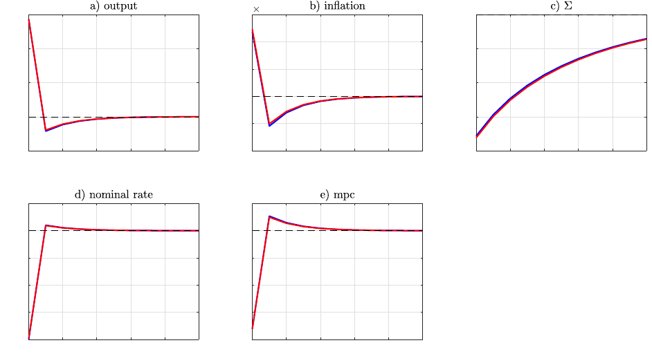
0 2 4 6 8 10
-0.02
0
0.02
0.04
0.06
0 2 4 6 8 10
-2
-1
0
1
2
3
10
-3
0 2 4 6 8 10
-0.04
-0.03
-0.02
-0.01
0
0 2 4 6 8 10
-0.2
-0.15
-0.1
-0.05
0
0.05
0 2 4 6 8 10
-0.2
-0.15
-0.1
-0.05
0
0.05
Figure 8. Time inconsistency with nominal debt: Optimal dynamics absent shocks in baseline calibration (κ = 0.01).
Blue line denotes HANK with countercylcical risk and real debt, red line denotes HANK with countercyclical risk and nominal
debt. All variables are plotted as percentage deviations from their steady state values.
.
18
